Chapter 28
Bipolar Transistors and Diodes
Bandgap references, temperature sensors and protection circuits all need junctions. SG13G2 offers fast SiGe HBTs and a substrate PNP; SKY130 offers fixed, characterized PNP and NPN cells built from its wells. This chapter reads their models, draws them with the PDKs' own generators, and shows that how they are sized, counted and placed decides how well they match.
- Describe the bipolar devices of a CMOS and a BiCMOS process, how each is built from the layer stack, and what the two PDKs offer.
- Read the Gummel plot, current gain, Early voltage and temperature behaviour of the SG13G2 HBTs and the SKY130 PNP and NPN cells from their models.
- Explain why ratios must be built from identical units, and choose a current density at which ΔVBE is PTAT.
- Estimate the random and systematic mismatch of a ratioed pair, and lay out a common-centroid 8:1 array with dummies that passes DRC.
- Use junction diodes and diode-connected bipolars in both PDKs, knowing their leakage, capacitance and the parasitic devices they bring with them.
Contents
Chapter 14 used the substrate PNP of each PDK to build a bandgap reference: it took \(V_{EB}\) as a CTAT voltage and the difference of two \(V_{EB}\) as a PTAT one, and designed the core around them. This chapter looks at the devices themselves. Which bipolar transistors and diodes does each PDK have, how are they built, what do their models say, and what does the layout have to do so that an 8:1 pair produces the PTAT voltage the circuit expects? The models are read and simulated in IIC-OSIC-TOOLS, the layouts come from IHP’s KLayout PyCells and from Magic’s SKY130 device generator, and a script builds and checks the matched arrays [35, 14, 20]:
python3 tools/layout/ch28/bjt_layouts.py      # PyCells and Magic draw the devices; 8:1 arrays; 3D model
python3 tools/layout/ch28/bjt_layouts.py drc  # KLayout DRC of the arrays and diodes (about a minute)
python3 tools/figs/_ch28_sim.py               # Gummel, temperature, Monte Carlo and diode runs, both PDKs (about a minute)
python3 tools/figs/ch28_bipolar.py            # the figures and tools/figs/ch28_numbers.json
Power bipolar transistors and ESD devices belong to Chapter 29; this chapter is about small-signal devices.
28.1 Bipolar devices in a CMOS and a BiCMOS process
What a layout can and cannot change
A bipolar transistor is two junctions back to back with a thin region between them. Forward-biasing the emitter–base junction injects minority carriers into the base; if the base is much thinner than the distance those carriers travel before they recombine, almost all of them reach the reverse-biased collector–base junction and are swept into the collector. The collector current is set by the emitter–base voltage alone:
Key equation · The bipolar transistor in its forward active region
\[I_C = I_S \exp\!\left(\frac{V_{BE}}{n V_T}\right)\left(1 + \frac{V_{CE}}{V_A}\right), \qquad I_S = J_S A_E + J_P P_E, \qquad \beta = \frac{I_C}{I_B}. \tag{28.1}\]\(V_T = kT/q\) is the thermal voltage (25.87 mV at 27 °C), \(n\) the ideality factor (close to 1), \(V_A\) the Early voltage. The saturation current \(I_S\) is the part a layout controls: a current density times the emitter area \(A_E\), plus a smaller term along its perimeter \(P_E\). The current gain \(\beta\), \(V_A\) and the speed are set by the vertical doping profile, which belongs to the process.
So the designer of a bipolar layout has fewer knobs than the designer of a MOS layout: the size and shape of the emitter, the number of emitters, and where they sit. Everything this chapter says about matching comes down to making \(I_S\) predictable through those three choices [61, 53]. The model equations behind Eq. (28.1) are those of Gummel and Poon, which the SKY130 bipolars and SG13G2’s substrate PNP use, and of VBIC, the extension that SG13G2’s HBTs use [129, 131].
Three structures
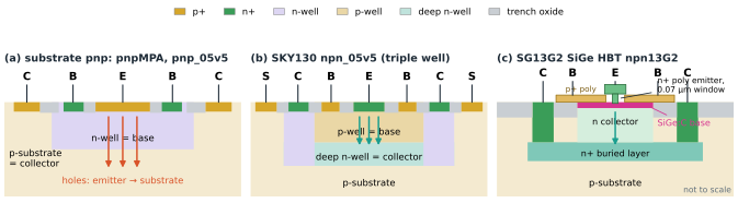
A CMOS process is designed around MOS transistors, yet it contains bipolar structures whether we want them or not. Figure 28.1 shows the three that matter here.
- The substrate PNP (a). A p+ diffusion in an n-well is the emitter, the n-well is the base and the p-type substrate is the collector. Every CMOS process has it, because every PMOS sits on exactly this stack. Its collector is the substrate, so it is always at ground; the device can only be used diode-connected (base and collector grounded, as in a bandgap) or as an emitter follower. SG13G2 calls it
pnpMPA, SKY130pnp_05v5. - The triple-well NPN (b). SKY130 has a deep n-well, an n-type layer buried under a p-well, which isolates NMOS transistors from the substrate. An n+ diffusion inside such an isolated p-well forms a vertical NPN: n+ emitter, p-well base, deep n-well collector, contacted through a ring of n-well. Its collector is free, but its base is a p-well designed for MOS transistors, not for bipolar gain. SKY130 calls it
npn_05v5. - The SiGe heterojunction bipolar transistor (c). A BiCMOS process adds the steps for a real bipolar transistor: an n+ buried layer as a low-resistance collector, an epitaxial base of silicon–germanium only a few tens of nanometres thick, and a polysilicon emitter that fills a narrow emitter window. The germanium content is graded across the base, which builds in a field that pushes electrons across it; this is what gives SG13G2’s
npn13G2its transit frequency of 300 GHz [15, 61].
What the two PDKs offer
Table 28.1 lists the bipolar devices of both PDKs with numbers from their models, and Figure 28.2 shows them as the generators draw them, all at the same scale. The SG13G2 devices are KLayout PyCells: the HBTs take a number of emitters Nx and an emitter length le, the substrate PNP any width and length. The SKY130 devices are fixed, characterized layouts: Magic places a copy of the cell from the sky130_fd_pr library, and the model card belongs to that exact layout [14, 18]. You can turn an HBT and a PNP of each PDK around in the 3D gallery.
Table 28.1. Bipolar devices of SG13G2 and SKY130, simulated at 27 °C with each PDK's typical models. β at its peak, n from the slope of the Gummel plot, VBE and its slope for the device diode-connected (base tied to collector) at 1 µA, and the local mismatch of IS per unit as written in the model card [14, 19].
| Device | Structure | Drawn emitter | β (peak) | \(n\) | \(V_{BE}\) at 1 µA | \(dV_{BE}/dT\) | σ(\(I_S\)) per unit |
|---|---|---|---|---|---|---|---|
SG13G2 npn13G2 |
SiGe HBT, VBIC | Nx × 0.07 × 0.9 µm, Nx = 1–10 | 800 | 1.023 | 0.665 V | −1.42 mV/K | 3.8 % |
SG13G2 npn13G2l |
SiGe HBT, low noise | Nx × 0.07 × le, le = 1–2.5 µm | 767 | 1.009 | 0.645 V | −1.46 mV/K | 3.8 % |
SG13G2 npn13G2v |
SiGe HBT, 2.5 V | Nx × 0.12 × le, le = 1–5 µm | 721 | 1.021 | 0.640 V | −1.46 mV/K | 3.8 % |
SG13G2 pnpMPA |
substrate PNP, Gummel–Poon | any W × L (2 × 2 µm here) | 1.1 | 1.016 | 0.719 V | −1.69 mV/K | not modelled |
SKY130 pnp_05v5_W0p68L0p68 |
substrate PNP | 0.68 × 0.68 µm, fixed | 14.0 | 1.043 | 0.743 V | −1.74 mV/K | 1.66 % |
SKY130 pnp_05v5_W3p40L3p40 |
substrate PNP | 3.4 × 3.4 µm, fixed | 14.5 | 1.009 | 0.680 V | −1.94 mV/K | not modelled |
SKY130 npn_05v5_W1p00L1p00 |
triple-well NPN | 1 × 1 µm, fixed | 36.7 | 1.040 | 0.717 V | −1.79 mV/K | 0.47 % |
SKY130 npn_05v5_W1p00L2p00 |
triple-well NPN | 1 × 2 µm, fixed | 34.4 | 1.041 | 0.702 V | −1.85 mV/K | 0.36 % |
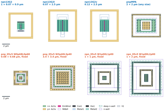
tools/layout/ch28/bjt_layouts.py.The figure makes one point about area at once. The emitter of npn13G2 covers 0.063 µm²; the cell around it, mostly its p+ substrate ring, covers 48 µm². SKY130’s 1 × 1 µm NPN needs a cell of 74 µm², because its collector is a deep n-well that must be contacted through an n-well ring, and that ring needs a p+ substrate ring around it. Of the eight devices drawn, only pnp_05v5_W3p40L3p40 spends more than a tenth of its cell on the emitter (26 %); pnpMPA at 2 × 2 µm spends 8 %.
Gummel plot and current gain
Figure 28.3a is the standard way to look at a bipolar transistor: collector and base current on a logarithmic axis against \(V_{BE}\), with the collector tied to the base so that \(V_{CB} = 0\). Over six to eight decades, \(I_C\) is a straight line whose slope is \(1/(nV_T)\), which is why bipolar transistors make such good logarithmic and exponential circuits and such good thermometers. \(I_B\) runs parallel to it in the middle; at low currents it bends upwards, because recombination in the emitter–base depletion region adds a base current with an ideality closer to 2; at high currents both curves bend down as the base fills with carriers (high injection) and the series resistances of emitter, base and collector take part of the applied voltage [53].
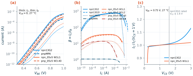
Panel (b) shows how differently the devices behave as transistors. The SG13G2 HBTs reach β = 720–800, inside the 300–1 200 range of the process specification, and their collector current at \(V_{BE}\) = 0.7 V, 3.7 µA, sits in the middle of the specified 2.6–5.2 µA [15]. SKY130’s NPN cells reach 37 and its PNP cells 14. SG13G2’s pnpMPA has β = 1.1: its model sends almost as much current into the base contact as into the substrate. For a diode-connected device in a bandgap that does not matter, since only the emitter current is forced and both base and collector go to ground; for anything that feeds the base it rules the device out.
28.2 The SG13G2 SiGe HBT
Three variants, one emitter window
All three SG13G2 HBTs share the structure of Figure 28.1c and differ in the emitter window and the collector doping [15]:
npn13G2, the fast device: a 0.07 × 0.9 µm emitter, repeatedNx= 1 to 10 times along the device; \(f_T\) 350 GHz typical (300 GHz minimum), \(f_{max}\) 450 GHz (400 GHz), \(BV_{CEO}\) 1.6 V (1.4 V).npn13G2l, a longer emitter of 1 to 2.5 µm for lower base resistance and noise, 1 to 4 emitters; \(f_T\) 330 GHz typical, the same breakdown.npn13G2v, a 0.12 µm emitter of 1 to 5 µm over a lighter collector: \(BV_{CEO}\) 2.5 V (2.2 V), \(f_T\) 120 GHz typical.
The models are VBIC subcircuits with four terminals, collector, base, emitter and the substrate node bn, plus an internal thermal node: VBIC models self-heating, the rise of the device’s own temperature with the power it dissipates. The thermal resistance of one npn13G2 emitter is 11 K/mW in the model card, so 100 µA at 1 V heats the device by 1.1 K and lowers its \(V_{BE}\) by 1.6 mV [14, 131]. Figure 28.3c shows the consequence. Between 0.8 and 1.4 V the collector current of a single emitter rises at a rate that corresponds to an Early voltage of only 62 V, although the card’s forward Early voltage is 189 V and the specification says 150 V: most of the extra slope is self-heating, the rest avalanche multiplication in the thin collector, which takes over above 2 V. For DC precision, keep \(V_{CE}\) and the current per emitter low, and give matched HBTs the same \(V_{CE}\); for RF, the rating of 1.6 V (2.5 V for npn13G2v) is a hard limit.
How IS scales with Nx and le
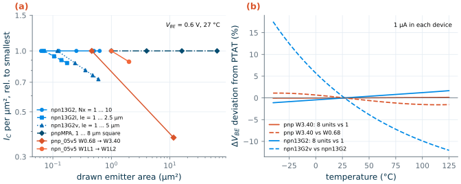
Figure 28.4a puts the scaling of Eq. (28.1) to the test: it plots the collector current per µm² of drawn emitter at \(V_{BE}\) = 0.6 V for every size the models accept, relative to the smallest. Adding emitters (Nx) scales \(I_S\) exactly, because the model multiplies every current by Nx. Lengthening the emitter does not: the per-area current of npn13G2l falls by 13 % from le = 1 to 2.5 µm and that of npn13G2v by 28 % from 1 to 5 µm. The model cards scale \(I_S\) as \(le^{0.85}\) and \(le^{0.8}\), a fit to measured devices in which the ends of the emitter stripe and lateral injection make a short emitter look relatively larger [14]. The rule follows directly: a current ratio is built by repeating one emitter, never by making one emitter longer.
Layout notes for the HBT
- The PyCell is the device. Its emitter window, base poly, collector contacts and substrate ring are drawn to the dimensions the model was extracted from; changing any of them by hand leaves the model behind. Matching therefore happens between whole PyCell instances, and the units of a matched set must have the same
Nxandleand the same orientation, with the emitter stripes parallel. - Multiple emitters share one collector. With
Nx> 1 the PyCell places the stripes 1.85 µm apart in one collector (Figure 28.2 showsNx= 1;Nx= 4 measures 12.3 × 7.1 µm). This saves area, but the outer emitters of such a device see different neighbours from the inner ones; for a precision ratio, use separateNx= 1 (or equal-Nx) instances arranged as a common centroid. - Self-heating is local. A matched HBT pair whose devices carry different currents or see different \(V_{CE}\) heats differently. Keep current densities equal; Section 28.4 shows how small a temperature difference matters.
- The minimum emitter matches poorly. The model’s 3.8 % random \(I_S\) variation per emitter means σ(ΔVBE) = 1.45 mV for a pair of single emitters (Section 28.4). Precision circuits use several emitters per device or the longer variants.
28.3 Parasitic PNP transistors in SKY130
The substrate PNP and its fixed cells
The substrate PNP of Figure 28.1a is the bipolar transistor of every CMOS bandgap. In SKY130 it comes in two characterized layouts (Figure 28.2): pnp_05v5_W0p68L0p68, a 0.68 µm square emitter, and pnp_05v5_W3p40L3p40, a 3.4 µm square emitter covered with contacts. Each has a ring of n+ tap on the n-well (the base contact), a p+ tap ring on the substrate (the collector contact) and the PDK’s marker layers. The cell is the device: the model card was fitted to that layout, and there is no parameter for any other size [18, 19].
Two consequences follow. First, the collector current flows into the substrate. The p+ ring of the cell collects it locally, but a reference that runs tens of microamperes through its PNPs pushes that current through the substrate resistance to the nearest ties, and a substrate that rises by a few tens of millivolts disturbs everything nearby. Give the PNPs generous substrate ties, as the cell’s own ring and the shared rings of Section 28.6 do, and keep them inside the guard-ring scheme of Chapter 24. Second, the two sizes are independent fits, not one model at two sizes. W0p68 has \(I_S\) = 1.51 aA, an ideality of 1.028, a temperature exponent \(X_{TI}\) = 1.1 and \(E_g\) = 1.20 eV; W3p40 has \(I_S\) = 7.12 aA, ideality 1.00, \(X_{TI}\) = 5.0 and \(E_g\) = 1.125 eV [19]. Their area ratio is 25, their \(I_S\) ratio 4.7, and the per-area current of Figure 28.4a drops to 0.37: the small emitter is dominated by its perimeter, the large one by its area.
Figure 28.4b shows what this does to a ΔVBE. Eight W3p40 units against one give a voltage that is PTAT within 0.13 % from −40 to 125 °C. One W3p40 against one W0p68 gives 63 mV at 27 °C, which looks like a generous ratio, but it bends away from PTAT by ±1.5 % over temperature, because the two cards have different \(X_{TI}\) and \(E_g\). The same experiment in SG13G2, npn13G2v against npn13G2, misses PTAT by up to 17 %. Even eight npn13G2 emitters against one tilt by 1–2 %, because VBIC gives the ideality factor a small temperature coefficient (TNF = 1.5 × 10⁻⁴ K⁻¹), which a bandgap trim absorbs as a slightly different slope.
What this means for your design
Count, do not stretch. A ratio of N is N copies of one unit cell, in the same orientation, at the same current density, never one larger cell or a cell of a different type. That holds for SKY130’s fixed PNPs, whose two sizes are separate models; for SG13G2’s HBTs, whose \(I_S\) scales with emitter length only as \(le^{0.8}\) to \(le^{0.85}\); and for SG13G2’s
pnpMPA, whose model scales with area alone while the silicon also has a perimeter term.
The triple-well NPN
SKY130’s npn_05v5 cells (Figure 28.2, bottom right) are the vertical NPN of Figure 28.1b in two sizes, 1 × 1 and 1 × 2 µm, and the four-terminal model includes the substrate node. Their β of about 36 is enough for a Brokaw-style bandgap, whose output is taken from the bases [79], and their \(I_S\) mismatch is the smallest in either PDK (0.47 % per device). The price is area: a 74 µm² cell for 1 µm² of emitter, a twentieth of the emitter area per µm² of cell that W3p40 achieves, and a deep n-well that brings its own spacing rules. The ideality of 1.04 also enters every ΔVBE directly.
SG13G2’s pnpMPA
SG13G2 draws its substrate PNP as a PyCell with any emitter width and length; Figure 28.2 uses 2 × 2 µm. The model is a Gummel–Poon card whose saturation current is 0.166 aA per µm² of emitter, with no perimeter term, and whose β is 1.1 independent of current [14]. It has an almost ideal exponential (n = 1.016) and the smallest curvature with temperature of all eight devices (Section 28.4), which makes it a good bandgap device in spite of its gain.
SG13G2 vs SKY130 · Substrate PNPs for references
SG13G2 pnpMPASKY130 pnp_05v5Emitter sizes any W × L (PyCell) 0.68 µm and 3.4 µm squares only Model one card, \(I_S\) ∝ area, β = 1.1 two independent cards, β ≈ 14 \(V_{EB}\) at 1 µA, slope 0.719 V, −1.69 mV/K (2 × 2 µm) 0.680 V, −1.94 mV/K (3.4 µm) Local mismatch in the model none W0p68: 1.66 % per device;W3p40: noneCell for a 4 µm² emitter 7.9 × 6.4 µm 6.7 × 6.7 µm for 11.6 µm² In SG13G2 you may choose a square emitter of any size, and 2 × 2 µm or more is a good unit for a bandgap. In SKY130 use
W3p40units for precision (Chapter 14 does) andW0p68only where area matters more than matching. SG13G2’s HBTs offer a free collector and high β where a circuit needs them.
28.4 Matching bipolar transistors for references
Temperature: the straight line and its curvature
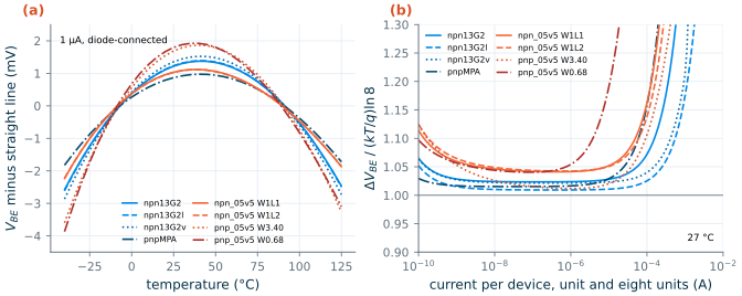
A bandgap uses \(V_{BE}\) as a CTAT voltage. Its slope at constant current, from Eq. (14.3), is \((V_{BE} - X_{TI}V_T - E_g/q)/T\); with the model parameters this gives −1.72 mV/K for pnpMPA and −1.92 mV/K for pnp_05v5_W3p40L3p40 at 1 µA, against −1.69 and −1.94 mV/K for straight-line fits to the simulations from −40 to 125 °C. But \(V_{BE}(T)\) is not a straight line: the \(X_{TI}V_T\ln T\) term bends it [130]. Figure 28.5a shows the residue after removing the best straight line, 2.8 mV peak to peak for pnpMPA, 3.4–4.4 mV for the HBTs and the SKY130 NPNs, and 5.5–5.8 mV for the SKY130 PNPs. A first-order bandgap cancels the slope and keeps this bow, which is the 10–30 ppm/K of curvature that Chapter 14 found; the straighter the device, the less a curvature correction has to do.
The PTAT voltage and its window
The PTAT voltage of eight identical units against one, both carrying the same current, is ideally \(nV_T\ln 8\). In a substrate PNP the circuit forces the emitter current, not the collector current, so a β that changes between the two current densities adds a term:
\[\Delta V_{BE} = V_{BE1} - V_{BE8} = nV_T\ln 8 + V_T\ln\frac{1 + 1/\beta_8}{1 + 1/\beta_1}. \tag{28.2}\]Figure 28.5b plots \(\Delta V_{BE}/(V_T\ln 8)\) against the current. Each device has a flat floor close to its own \(n\): 1.009 to 1.024 for the HBTs, 1.015 for pnpMPA, 1.012 for W3p40 and 1.04 for the SKY130 NPNs and W0p68. At high currents the series resistances and high injection of the single unit, which carries eight times the current density of the others, raise the ratio steeply. At very low currents the recombination part of the base current, which changes β with current, and leakage raise it again. The usable window, where the ratio stays within 1.5 % of its floor, runs from about 10 nA to 10 µA per device for the HBTs, pnpMPA and W3p40, but only up to about 1 µA for W0p68. Hastings recommends staying well below the point where the Gummel plot leaves its straight line, because that point moves with the process [61]; Figure 28.5b shows where it is in each PDK.
Worked example 28.1 · VEB, its slope and ΔVBE of an 8:1 pair, by hand and by simulation
SG13G2, pnpMPA 2 × 2 µm at 1 µA. \(I_S\) = 0.166 aA/µm² × 4 µm² = 0.664 aA at 27 °C (the card’s TNOM). With β = 1.1 the emitter current of 1 µA splits into \(I_C\) = 1 µA × 1.1/2.1 = 0.524 µA. Then \(V_{EB} = nV_T\ln(I_C/I_S)\) = 1.015 × 25.87 mV × ln(0.524 µA/0.664 aA) = 26.25 mV × 27.39 = 0.7192 V; the simulation gives 0.7193 V. The slope from Eq. (14.3) with \(X_{TI}\) = 2.54 and \(E_g\) = 1.17 eV is (0.7192 − 2.54 × 0.02587 − 1.17)/300.15 K = −1.72 mV/K (simulated −1.69 mV/K as a straight line over the whole range). Since β does not change with current, Eq. (28.2) reduces to \(nV_T\ln 8\) = 1.015 × 25.87 × 2.079 = 54.6 mV, rising by 0.182 mV/K; the simulation gives 54.7 mV and 0.182 mV/K.
SKY130, pnp_05v5_W3p40L3p40 at 1 µA. The card’s \(I_S\) of 7.12 aA is given at its TNOM of 30 °C; the Gummel plot of Figure 28.3 gives 3.84 aA at 27 °C. β = 14.25 at 1 µA, so \(I_C\) = 0.934 µA and \(V_{EB}\) = 25.87 mV × ln(0.934 µA/3.84 aA) = 25.87 × 26.22 = 0.678 V (simulated 0.680 V). Slope: (0.678 − 5.0 × 0.02587 − 1.125)/300.15 = −1.92 mV/K (simulated −1.94). ΔVBE: \(V_T\ln 8\) = 53.8 mV; β falls from 14.25 at 1 µA to 13.2 at the 125 nA of each of the eight units, which Eq. (28.2) turns into +0.14 mV. The simulation gives 54.4 mV: within 1.2 % of the ideal value, the rest coming from the low-current base current of the card.
What it means. For the 8:1 ratio of a bandgap, 1 µA per device sits in the flat part of Figure 28.5b in both PDKs, and the hand formulas predict the PDK models to a few tenths of a percent. The ideality factor matters more than it seems: SKY130’s NPN would give 4 % more PTAT voltage than \(V_T\ln 8\), and a bandgap designed with the ideal value would land off its zero-TC point.
Random mismatch: σ(ΔVBE) from σ(IS)
Two identical units at the same current differ in \(V_{BE}\) because their saturation currents differ. From Eq. (28.1), a relative error in \(I_S\) becomes a voltage error through the logarithm:
Key equation · Random VBE mismatch
\[\sigma(\Delta V_{BE}) = nV_T\,\sigma\!\left(\frac{\Delta I_S}{I_S}\right), \qquad \sigma\!\left(\frac{I_S}{I_S}\right)_{\text{unit}} = \frac{A_{IS}}{\sqrt{A_E}}, \qquad \sigma(\Delta V_{BE})_{1:N} = nV_T\,\sigma_{\text{unit}}\sqrt{1 + \tfrac{1}{N}}. \tag{28.3}\]\(A_{IS}\) (%·µm) is a Pelgrom coefficient for the saturation current of one device. A pair has \(\sqrt 2\) times the unit σ; a 1 : N pair has \(\sqrt{1 + 1/N}\) times, because the N units average.
This is why bipolar transistors are prized for matching: the exponential turns a 1 % error in \(I_S\) into only 0.26 mV [61, 75]. Figure 28.6a shows Monte Carlo runs of 200 pairs and 200 8:1 sets of each device whose model carries local mismatch, with the hand values of Eq. (28.3) as black bars. A pair of single npn13G2 emitters has σ = 1.45 mV (hand 1.39 mV), an 8:1 set of them 1.07 mV (1.04 mV); W0p68 pairs 0.62 mV and 8:1 sets 0.47 mV; npn_05v5_W1p00L1p00 pairs 0.17 mV. Turned into \(A_{IS}\), the cards say 0.95 %·µm for the HBT emitter, 1.13 %·µm for W0p68 and 0.47 %·µm for SKY130’s NPN: within a factor of 2.5 of each other, so the small emitters match poorly mainly because they are small.
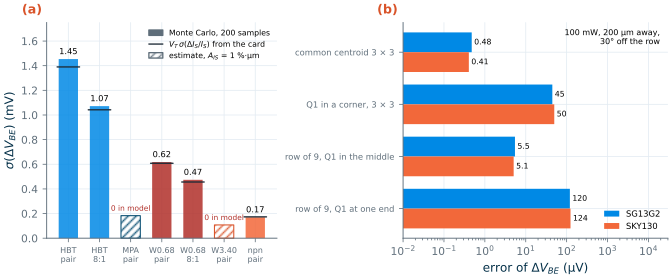
hbt_typ_mismatch with mm_ok=1, SKY130 tt_mm), 200 samples (±5 %); black: Eq. (28.3) with the card's σ(IS). Hatched: our estimate for the two PNPs without a mismatch model, AIS = 1 %·µm. (b) Systematic error of the PTAT voltage of the 8:1 arrays of Section 28.6 (unit pitch of each PDK) and three other placements, in the field of a 100 mW point source 200 µm away and 30° off the row, using each PNP's dVEB/dT.Common pitfall · A Monte Carlo that says your bandgap PNPs are perfect
The two PNPs a bandgap is most likely to use, SG13G2’s
pnpMPAand SKY130’spnp_05v5_W3p40L3p40, carry no local mismatch in their models:pnpMPAhas no mismatch parameter at all, and the mismatch terms ofW3p40are multiplied by a slope parameter that the library sets to zero [14, 19]. A Monte Carlo run of a bandgap built from them returns the amplifier’s and the resistors’ contributions and nothing from the bipolars, which is too optimistic. Add the bipolar part by hand with Eq. (28.3), or put an explicit offset source in series with Q1 in the testbench, using an \(A_{IS}\) of about 1 %·µm as the modelled devices of both PDKs suggest; the foundry’s matching data, where available, replace this estimate.
Worked example 28.2 · How much of a bandgap’s spread comes from its bipolars?
A voltage-mode bandgap (Chapter 14) has \(V_{REF} = V_{EB3} + (R_2/R_1)\Delta V_{BE}\) with \(R_2/R_1 \approx 10\), so any error in ΔVBE appears ten times larger at the output.
SG13G2, pnpMPA 2 × 2 µm, 8:1. With \(A_{IS}\) = 1 %·µm, one unit varies by 1 %/2 µm = 0.50 %. Eq. (28.3): σ(ΔVBE) = 25.87 mV × 0.005 × √(1 + 1/8) = 0.137 mV, so σ(VREF) ≈ 1.4 mV, 0.11 % of 1.2 V.
SKY130, pnp_05v5_W3p40L3p40, 8:1. One unit: 1 %/3.4 µm = 0.29 %; σ(ΔVBE) = 25.87 × 0.0029 × 1.06 = 0.081 mV, σ(VREF) ≈ 0.8 mV.
With minimum devices. An 8:1 set of single
npn13G2emitters gives 1.04 mV by hand and 1.07 mV by Monte Carlo, about 11 mV at the output;W0p68gives 0.46 mV by hand and 0.47 mV by Monte Carlo, about 5 mV at the output.Compared with the amplifier. The error amplifier’s input offset adds to ΔVBE directly and is multiplied by the same factor of about ten. The OTAs of Chapter 13 have random offsets of 0.9 to 2.2 mV, ten times more than the 2 × 2 µm or 3.4 µm PNP arrays. With such units the bipolars are not what limits an untrimmed bandgap; with minimum emitters they are.
Systematic mismatch: temperature, stress and the layout
A bipolar pair is a good thermometer, and that is its weakness as a matched pair. With \(dV_{BE}/dT\) ≈ −1.7 to −1.9 mV/K, a temperature difference of only 0.1 K between Q1 and the units of Q2 shifts ΔVBE by 0.17–0.19 mV, more than the random σ of a good array [61]. Figure 28.6b evaluates the gradient model of Chapter 27 (Eq. 27.5 in the field of Eq. 27.6) for the real unit positions of the 8:1 arrays of Section 28.6 and three other placements, near a 100 mW source 200 µm away. With Q1 at one end of a row of nine, the error is 120 µV, the same sign on every chip; with Q1 in a corner of the 3 × 3 block, 45–50 µV; with Q1 in the middle of the row, 5 µV; with Q1 in the centre of the 3 × 3 block, the common centroid, under 0.5 µV. The linear part of the field cancels exactly and only the curvature remains, which the square block keeps small because it is compact.
Mechanical stress is the other systematic effect. Silicon’s band structure changes under stress, so \(I_S\) and with it \(V_{BE}\) shift: the piezojunction effect. Packaging puts the die under stress that is largest at its edges and corners. Hastings reports that on (100) silicon a vertical PNP is about three times less sensitive to in-plane stress than a vertical NPN, one more reason why substrate-PNP bandgaps are popular, and that placing the matched devices near the centre of the die or on one of its axes of symmetry, away from heat sources, minimizes both kinds of gradient [61]. Neither PDK models stress in its bipolars.
Rules for matched bipolar transistors
Collecting the points of this chapter, with Hastings’s rules for vertical transistors as the checklist [61]:
- Identical units. The same cell (SKY130), the same PyCell parameters (SG13G2), the same orientation; ratios by count, never by size or type (Figure 28.4).
- Square, generous emitters. A square has the most area for its perimeter, so the less predictable perimeter term weighs least; size the unit from Eq. (28.3) for the σ the circuit needs.
- Common centroid, compact. For 1 : 8, the 3 × 3 block with the single unit in the centre; for equal pairs, the cross-coupled quad of Chapter 27. Keep the group small, because the residue of a curved field grows with its span.
- Dummies around the group, at the same pitch, so that every active unit sees the same surroundings, and connected (emitter to base, Section 28.6).
- Equal current densities, equal voltages. Keep every unit inside the PTAT window of Figure 28.5b and at the same \(V_{CB}\) (it is zero for diode-connected units; in a Brokaw cell or a mirror use cascodes).
- Identical contacts and metal. The same number and position of emitter contacts in every unit, because contacts inside the emitter change β; base and collector contacts symmetric around each emitter; the same metal over every unit.
- Separate emitters in a shared base far enough apart. If several emitters sit in one base region, space them at the rule for unconnected emitters plus a margin, so that their depletion regions and lateral currents do not interact.
- Away from heat sources and die edges, on an axis of symmetry of the heat sources, with a substrate ring around the group.
28.5 Diodes
Junction diodes in the two PDKs
A junction diode is a single pn junction with an anode and a cathode contact. Both PDKs provide the two kinds a CMOS process makes naturally (Figure 28.7): an n+ diffusion in the p-type substrate or p-well (SG13G2 dantenna, SKY130 diode_pw2nd_05v5) and a p+ diffusion in an n-well (SG13G2 dpantenna, SKY130 diode_pd2nw_05v5). Both serve as antenna diodes, which protect gates from the charge that collects on long wires during plasma etching (Chapter 24), and their models are close relatives of the drain and source junctions that every transistor has anyway. SG13G2 also has a Schottky diode, schottky_nbl1, which uses the HBT’s buried layer as its cathode [15].
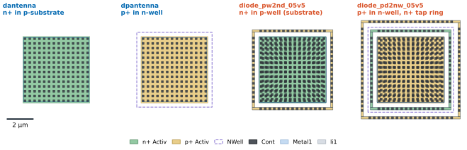
dantenna, dpantenna and Magic's diode_pw2nd_05v5, diode_pd2nw_05v5. The SKY130 diodes pass the KLayout rule deck as drawn; the bare dantenna fails the latch-up rule LU.b, which asks for a substrate tie close to every n+ region outside a well.Figure 28.8 and Table 28.2 compare the four diodes at the same drawn size. The most striking number is SKY130’s n+/p-well diode: at 0.6 V forward it conducts 3.6 µA, 70 times more than SG13G2’s n+/p-substrate diode, with an ideality of 1.29. SKY130’s p+/n-well diode has an ideality of 1.36. Such idealities say that the forward current is not the clean diffusion current of Eq. (28.1); the cards were fitted for leakage and capacitance, which is what the junctions of transistors need, not for forward precision. SG13G2’s two diodes have idealities of 1.02–1.03 and are closer to the bipolar devices.
Table 28.2. Junction diodes of 5 × 5 µm in SG13G2 (VDD = 1.2 V) and SKY130 (VDD = 1.8 V), simulated with the typical models [14, 19]. Reverse currents with ngspice's minimum conductance set to 10⁻¹⁸ S (its default of 1 pS across each junction would hide them).
| Quantity | SG13G2 dantenna |
SG13G2 dpantenna |
SKY130 diode_pw2nd_05v5 |
SKY130 diode_pd2nw_05v5 |
|---|---|---|---|---|
| Junction | n+ / p-substrate | p+ / n-well | n+ / p-well | p+ / n-well |
| Forward current at 0.6 V | 50 nA | 25 nA | 3.6 µA | 260 nA |
| Ideality \(n\) | 1.03 | 1.02 | 1.29 | 1.36 |
| \(V_F\) at 1 µA, slope | 0.696 V, −1.85 mV/K | 0.710 V, −1.76 mV/K | 0.558 V, −2.06 mV/K | 0.647 V, −3.16 mV/K |
| Reverse current at −VDD, 27 / 85 / 125 °C | 90 / 356 / 728 pA | 0.13 fA / 11 fA / 0.36 pA | 0.06 / 19 / 477 pA | 0.01 / 18 / 972 pA |
| Capacitance at 0 V / −VDD | 23.8 / 17.7 fF | 21.4 / 15.5 fF | 34.2 / 20.1 fF | 20.4 / 13.1 fF |
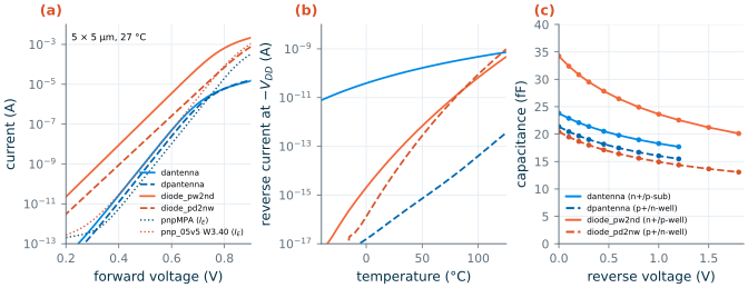
Leakage, panel (b), is thermal generation in the depletion region and diffusion from the neutral regions, and it grows steeply with temperature: the SKY130 diodes leak 0.5 and 1 nA at 125 °C, about ten times more for every 25 K. For a sample-and-hold switch (Chapter 19) or a high-impedance bias node, these are the numbers that set the droop at high temperature, and they scale with junction area. SG13G2’s dantenna is the exception that needs care: its reverse current comes almost entirely from the breakdown term of its area model (BV = 11.6 V with a very soft knee, NBV = 48.9) and rises only eightfold from 27 to 125 °C [14]. It is best read as a pessimistic bound fitted for an antenna diode, not as a leakage model. The capacitance, panel (c), follows the junction law of Chapter 26: 0.8–1.4 fF per µm² of diode at zero bias, perimeter included, falling by a quarter to 40 % at −VDD.
The parasitic devices every diode brings
A junction in a CMOS substrate is never alone, and each of the four diodes is part of a bipolar transistor:
- A p+/n-well diode is the emitter–base junction of a substrate PNP. Forward-biased, it injects holes into the n-well, and the substrate collects most of them: a fraction β/(β+1) of the forward current, 93 % in SKY130 (β ≈ 14) and 52 % with SG13G2’s
pnpMPAcard (β = 1.1). That current flows to ground through the substrate, not out of the cathode. The diode modelsdpantennaanddiode_pd2nw_05v5do not contain this transistor; the PNP models do. Whenever a p+/n-well diode can conduct, simulate it as a PNP. - An n+/p-substrate diode is the emitter of a lateral NPN. Forward-biased, it injects electrons into the substrate, and any n-well within reach, the n-well of a PMOS for instance, collects them as a collector. That current is one half of the trigger of latch-up (Chapter 24), which is why the rule deck’s LU.b asks for a substrate tie next to the bare
dantennaof Figure 28.7, and why guard rings surround any junction that might be forward-biased. - Every transistor drain and source is such a diode. An output pin that swings below ground or above the supply forward-biases them; the protection devices that handle this deliberately are the subject of Chapter 29.
Diodes for temperature sensing and protection
A temperature sensor needs a junction whose voltage follows the exponential law with a known ideality, and Table 28.2 shows that SKY130’s junction diodes are not that: an ideality of 1.29–1.36 that the model does not tie to physics, and slopes of −2.1 and −3.2 mV/K at 1 µA. Use a diode-connected bipolar instead, the substrate PNP in either PDK. Better still, measure ΔVBE of one device at two currents, I and 8I in turn, instead of \(V_{BE}\): the difference is \(nV_T\ln 8\) whatever \(I_S\) is, so neither the absolute value of \(I_S\) nor the mismatch of two devices enters, and a sigma-delta converter can digitize it against a bandgap made of the same transistors. This is how precision CMOS temperature sensors are built [132, 69]. Two corrections remain: the ideality, which Table 28.1 gives for each device, and the series resistance of the base, which adds a current-dependent term and is cancelled by measuring at three currents or keeping the currents low.
As protection devices, diodes are used reverse-biased, as clamps that conduct only when a node goes beyond a supply. Their cost to the circuit is the capacitance and leakage of Table 28.2, and their danger is the injection described above whenever they do conduct. For matching, junction diodes follow the rules of Section 28.4: identical units, square shapes, a common centroid, equal currents.
28.6 Layout of a bandgap core
An 8:1 array from the PDK cells
Figure 28.9 is the bipolar part of the bandgaps of Chapter 14, drawn in both PDKs by bjt_layouts.py. Each is a 5 × 5 grid of one unit cell, IHP’s pnpMPA PyCell with a 2 × 2 µm emitter or SkyWater’s pnp_05v5_W3p40L3p40 cell, unmodified. The inner 3 × 3 block is the ratioed pair: Q1 in the centre, the eight units of Q2 around it, so that Q1 and Q2 share their centroid and the group is as compact as a 1 : 8 group can be. The outer ring of 16 units are dummies. The construction follows the rules of Section 28.4:
- Shared substrate rings. The units are abutted so that their collector rings, all at ground, merge. In SG13G2 the rings overlap completely, a pitch of 7.15 × 5.67 µm, because the PyCell places the ring contacts on a common grid; in SKY130 the rings abut at a pitch of 6.44 µm, because overlapping them would merge contacts that are not on a common grid and break the contact-size rule. The outer rings of the dummies form one continuous substrate ring around the array.
- Diode connection in each unit. A short strip of first metal (SG13G2) or li1 (SKY130) on the left and on the right of every unit ties its base ring to its collector ring, so every unit, dummy or not, is the diode-connected PNP of the bandgap, with identical surroundings.
- Dummies off. Each dummy’s emitter is tied to its base by a strip at the top, so the dummies carry no current but look like the active units to lithography, implantation and heat flow.
- Symmetric emitter routing. Q2’s eight emitters are joined on the second metal: one track along each of the two outer rows of the block, two stubs from the middle row out to two vertical spines over the dummy columns, and a bar below the array. Q1’s emitter goes up through a via stack to the third metal and runs straight up and down the centre column, crossing Q2’s tracks only on another layer. The routing is mirror-symmetric about both axes of the array.
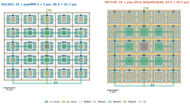
pnpMPA 2 × 2 µm, 36.5 × 31.7 µm. SKY130: 25 × pnp_05v5_W3p40L3p40, 32.5 × 35.2 µm. Both pass their PDK's KLayout rule deck with zero violations (IHP run_drc.py without the density checks; SKY130 sky130A_mr.drc). Generated by tools/layout/ch28/bjt_layouts.py.Only 9 of the 25 units carry current, so the arrays spend almost two thirds of their area on dummies. That is the normal price of a precision 1 : 8 group; a less critical reference might use a single ring of dummies only where the array has open sides, or none. The emitter area per array is 36 µm² (SG13G2) and 104 µm² (SKY130), and Worked example 28.2 shows that this is enough for the bipolars to stay well below the amplifier’s share of the error. The SKY130 array is shown in 3D below; hide met3 and met2 to see the emitters, and li1 to see how each unit’s base ring is strapped to the shared substrate ring.
SkyWater's fixed pnp_05v5_W3p40L3p40 cells, placed and routed by tools/layout/ch28/bjt_layouts.py; 820 kB.
Floorplan of the core
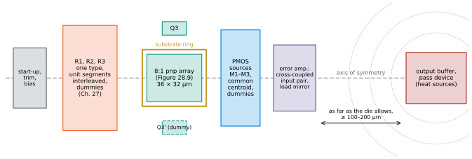
The bipolar array is one block of the bandgap core. Figure 28.10 arranges the others around it along one axis of symmetry: the resistor array of \(R_1\), \(R_2\) (and \(R_3\) in the current-mode core), built from unit segments of one resistor type and interleaved as in Chapter 27; the PMOS current sources as a common centroid with dummies; the error amplifier with a cross-coupled input pair; and the start-up, trim and bias circuits at the far end. The third bipolar of the voltage-mode core, Q3, sits on the axis next to the array, and a dummy in the mirror position keeps the array’s surroundings symmetric. The heat sources of the chip, an output buffer or the pass device of a regulator, go on the same axis as far away as the die allows, so that their isotherms are symmetric about the array and the gradient along the axis falls on a common-centroid group that cancels it.
A checklist for the bipolar part of a reference
- Are Q1 and Q2 built from identical units of one cell, with Q2 = N copies, and is each unit inside the PTAT window of Figure 28.5b at its bias current?
- Is the random σ(ΔVBE), multiplied by the core’s gain \(R_2/R_1\), small next to the amplifier’s offset times the same gain? If the model has no mismatch (
pnpMPA,W3p40), was it added by hand? - Is the group a common centroid (3 × 3 for 1 : 8, cross-coupled for 1 : 1), surrounded by connected dummies, with symmetric routing?
- Is every unit diode-connected in the same way, with the same contacts and metal over it?
- Are the substrate ties generous enough for the collector currents, and is the array inside a substrate ring?
- Is the array on an axis of symmetry of the heat sources, far from them, away from the die edges and corners?
- In SG13G2 with HBTs: equal
Nxandle, equal current densities and \(V_{CE}\), and \(V_{CE}\) within the device’s rating?
Try it · Smaller units, more current, your own placement
In
tools/layout/ch28/bjt_layouts.py, set the SKY130 unit to the small PNP (cell="pnp_w0p68"inTECH["sky130"]) and runpython3 tools/layout/ch28/bjt_layouts.py build export drc: the script reads the cell’s rings and emitter, finds the pitch and redraws the array. How much smaller is it, does it still pass the rule deck, and what does Worked example 28.2 say about its σ(ΔVBE) with the card’s 1.66 %? Intools/figs/_ch28_sim.py, setI_UNIT = 10e-6and rerun it andpython3 tools/figs/ch28_bipolar.py temp: which devices leave the PTAT window? Finally, add your own arrangement of Q1 and the eight units of Q2 toplacements()intools/figs/ch28_bipolar.py(a 2 × 5 block, say) and runpython3 tools/figs/ch28_bipolar.py mismatchto see what error the hot spot leaves.
- A CMOS process always contains a substrate PNP (p+ emitter, n-well base, substrate collector); SKY130 adds a triple-well NPN and SG13G2 three SiGe HBTs with β of 700–800 and fT up to 350 GHz. The layout controls only the emitter’s size, number and position; β, VA and speed belong to the process.
- SKY130’s bipolars are fixed cells with independent model cards (the two PNPs differ in IS per area by 2.7 times and in XTI by 5 : 1.1); SG13G2’s HBT IS scales exactly with the number of emitters but only as le0.8–le0.85 with length. Build every ratio from identical units; only then is ΔVBE PTAT.
- VBE falls by 1.4–1.9 mV/K and is bowed by 3–6 mV over −40 to 125 °C; ΔVBE equals nVT ln N, with n = 1.01–1.04, inside a window of about 10 nA to 10 µA per device (1 µA for SKY130’s small PNP).
- σ(ΔVBE) = nVT σ(ΔIS/IS), with AIS ≈ 0.5–1.1 %·µm in the models; minimum HBT emitters give 1.45 mV per pair, but
pnpMPAandW3p40have no mismatch model at all. A 0.1 K difference costs as much as the random part: use a compact common centroid with dummies, away from heat sources.- Junction diodes differ by orders of magnitude between the PDKs in forward current and leakage (SKY130 n+/p-well: n = 1.29, 0.5 nA at 125 °C for 25 µm²); a forward-biased p+/n-well diode is a substrate PNP that sends 93 % of its current into the substrate. For temperature sensing use a diode-connected bipolar and ΔVBE at two currents.
- The 8:1 arrays of this chapter (36.5 × 31.7 µm in SG13G2, 32.5 × 35.2 µm in SKY130) are built from unmodified PDK cells with shared substrate rings, per-unit diode connections, 16 dummies and symmetric routing, and pass both rule decks.
Further reading
- R. A. Hastings, The Art of Analog Layout [61], Chapter 9 (bipolar transistors in CMOS and BiCMOS processes, including SiGe HBTs), Sections 10.2–10.3 (matching bipolar transistors, the piezojunction effect and rules for matching) and Sections 11.2–11.3 (diodes in CMOS and BiCMOS and their matching).
- P. R. Gray, P. J. Hurst, S. H. Lewis and R. G. Meyer [53], Chapter 1: the bipolar transistor model behind Eq. (28.1), with its high-injection and base-resistance effects.
- Y. P. Tsividis [130]: the exact temperature dependence of VBE and why a first-order bandgap keeps its curvature.
- G. C. M. Meijer, G. Wang and F. Fruett [132], and M. A. P. Pertijs and J. H. Huijsing [69]: substrate PNPs as temperature sensors and references in CMOS, with the ΔVBE techniques of Section 28.5.
- The bipolar sections of the PDK model libraries,
sg13g2_hbt_mod.lib(VBIC cards of the HBTs and thepnpMPAcard) for SG13G2 [14] and thepnp_05v5andnpn_05v5cards ofsky130_fd_pr[19], and the SG13G2 process specification for the HBTs’ ratings [15].