Chapter 7
Single-Transistor Amplifiers
Three ways to connect one transistor (common source, common gate and common drain) give three amplifiers with very different gain and impedances. Cascoding combines them, and shows most clearly how differently the two PDKs behave.
- Analyse the common-source stage with resistive, diode and current-source loads, and explain the trade-off between gain and output swing.
- Use source degeneration to trade transconductance for linearity.
- Analyse the source follower and the common-gate stage, including the body effect and the input and output resistances.
- Explain how a cascode raises output resistance, what headroom it costs, and design a telescopic cascode stage to a gain specification in both PDKs.
Contents
Every amplifier in this book is built from a handful of one-transistor stages. A transistor has three useful terminals, and the stage is named after the terminal that is shared by the input and the output: in a common-source (CS) stage the input drives the gate and the output is taken from the drain; in a common-gate (CG) stage the input drives the source; and in a common-drain stage, better known as the source follower, the output is taken from the source.
To keep the chapter concrete, we reuse one transistor throughout: the input device \(M_1\) of Worked example 6.1. It was sized for \(g_m = 628\ \mu\mathrm{S}\) at \(g_m/I_D = 15\ \mathrm{V^{-1}}\), so it carries \(I_D = 41.9\ \mu\mathrm{A}\); in SG13G2 it is 18.05/0.75 µm (two fingers), in SKY130 4.62/0.18 µm. In Chapter 6 it drove an ideal current source. Here we change what surrounds it, one connection at a time, and watch what happens to gain, swing and impedance. All numbers come from the lookup tables of Section 6.4 and from ngspice runs of tools/figs/ch07_single_stage.py, at the tt corner and 27 °C. The small-signal analysis follows the classic textbooks [51, 53, 7]; the gm/ID view of it follows Jespers and Murmann [56].
7.1 Common source with a resistive load
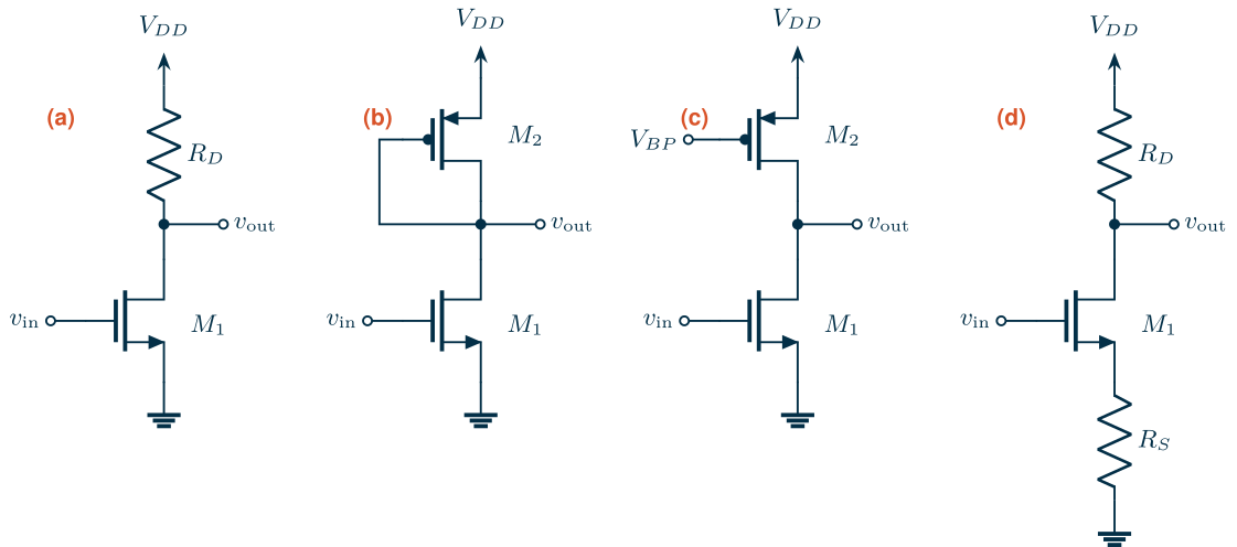
The physical idea is simple. A small change \(v_{in}\) of the gate voltage changes the drain current by \(g_m v_{in}\). That current flows through the load resistor \(R_D\) in Figure 7.1(a), and through the transistor’s own output resistance \(r_o = 1/g_{ds}\), which is in parallel with it. The output voltage moves the opposite way to the input, so the gain is negative:
\[A_v = \frac{v_{out}}{v_{in}} = -g_m\,(R_D \parallel r_o). \tag{7.1}\]Eq. (7.1) makes the gain look like a free choice: pick a large \(R_D\). But \(R_D\) also carries the bias current, and the voltage it drops, \(V_{RD} = I_D R_D\), must fit inside the supply. Write \(g_m\) as \((g_m/I_D)\cdot I_D\), and the output resistance through the Early voltage, which the lookup tables give directly from the intrinsic gain and \(g_m/I_D\):
\[V_A = \frac{I_D}{g_{ds}} = \frac{g_m/g_{ds}}{g_m/I_D}, \qquad r_o = \frac{V_A}{I_D}. \tag{7.2}\]The bias current then cancels out:
Key equation · Gain of a resistively loaded stage
\[\lvert A_v\rvert = \frac{(g_m/I_D)\cdot V_{RD}}{1 + V_{RD}/V_A}. \tag{7.3}\]The gain is set by two voltages and the inversion level, not by the size of anything. To double the gain you must double the voltage across the resistor.
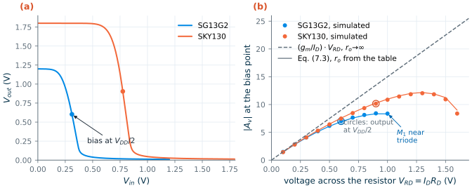
With \(g_m/I_D = 15\ \mathrm{V^{-1}}\) and the output at \(V_{DD}/2\), an ideal transistor would give \(15 \times 0.6 = 9\) in SG13G2 and \(15\times 0.9 = 13.5\) in SKY130. The tables give \(V_A\) = 2.0 V for the SG13G2 device (L = 0.75 µm) and 2.9 V for the SKY130 device (L = 0.18 µm) at \(V_{DS} = V_{DD}/2\), which brings the predictions down to 6.9 and 10.3.
Figure 7.2 checks this. Panel (a) shows the transfer curves with \(R_D\) = 14.3 kΩ and 21.5 kΩ, chosen to put the output at \(V_{DD}/2\) for the 41.9 µA bias. The simulated gains at that point are 7.0 and 10.2, within 1 % of Eq. (7.3). Panel (b) repeats the simulation for every resistor drop from 0.1 V upwards, each time re-biasing the gate so that the current stays at 41.9 µA. The gain grows almost linearly with \(V_{RD}\), exactly as Eq. (7.3) says, until the output gets so low that \(M_1\) approaches the triode region: then its \(r_o\) and \(g_m\) collapse and the gain falls again. The best SG13G2 can do is 8.4 at \(V_{RD}\approx 0.9\) V; SKY130 reaches 12.0 at 1.3 V.
What this means for your design
A resistively loaded stage in a 1.2 V process cannot have a gain much above 10, whatever you do with sizes. Use it where a modest, well-defined, linear gain is wanted and where a resistor is welcome anyway, for example as a wideband pre-amplifier. For high gain the load must have a high small-signal resistance while dropping a small DC voltage. Only a transistor can do that.
7.2 Active loads
Replacing the resistor with a transistor gives two very different loads, shown in Figure 7.1(b) and (c).
The diode-connected load
A transistor with its gate tied to its drain is always in saturation, and a small-signal voltage across it changes the current through it by \(g_{m2}\) per volt (plus a little \(g_{ds2}\)). It behaves like a resistor of value \(1/g_{m2}\). The gain is
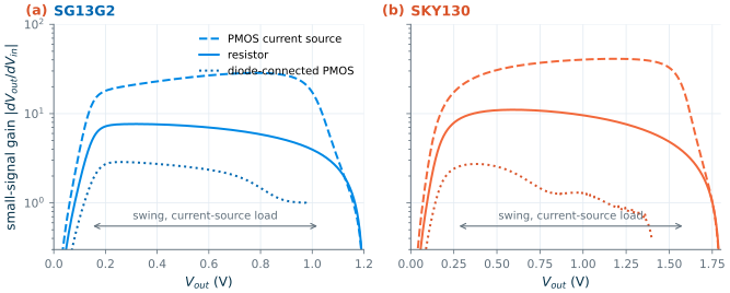
\[\lvert A_v\rvert = \frac{g_{m1}}{g_{m2} + g_{ds1} + g_{ds2}} \approx \frac{(g_m/I_D)_1}{(g_m/I_D)_2}, \tag{7.4}\]where the last step uses the fact that \(M_1\) and \(M_2\) carry the same current. This is a lovely result: the gain is the ratio of two inversion levels, independent of the process, the current and the device sizes. With \(M_1\) at 15 V⁻¹ and the PMOS load sized for 5 V⁻¹ (L = 0.5 µm), we expect a gain of 3. The simulated gain is 2.65 in both PDKs; the 12 % shortfall is the \(g_{ds1} + g_{ds2}\) term in Eq. (7.4), which we dropped.
The price is headroom. A low \(g_m/I_D\) for \(M_2\) means a large overdrive, and the load’s \(V_{SG}\) comes straight off the output’s DC level. The SG13G2 PMOS needs 0.745 V and the SKY130 PMOS, whose threshold is near 1 V, needs 1.34 V. Both outputs sit at about 0.46 V. For a gain of 5 you would need the load at 3 V⁻¹, a gate voltage that does not fit in either supply.
The current-source load
A PMOS transistor with a fixed gate voltage \(V_{BP}\) delivers a nearly constant current, so its small-signal resistance is its own \(r_{o2}\), while it drops only a few hundred millivolts. The gain is
\[\lvert A_v\rvert = \frac{g_{m1}}{g_{ds1} + g_{ds2}} = g_{m1}\,(r_{o1}\parallel r_{o2}). \tag{7.5}\]With an ideal current source, \(g_{ds2} = 0\) and Eq. (7.5) is the intrinsic gain of Chapter 6. We size the PMOS as a current source, at \(g_m/I_D = 10\ \mathrm{V^{-1}}\) and L = 1 µm (W = 30.9 µm in SG13G2, 35.9 µm in SKY130). The tables give \(g_{ds2}\) = 3.0 µS and 1.15 µS against \(g_{ds1}\) = 20.6 µS and 14.7 µS, so the predicted gains are 26.2 and 39.8. Simulation gives 26.8 and 39.3.
Gain against swing
Figure 7.3 compares the three loads in the way that matters for a design: the small-signal gain at every point of the transfer curve, plotted against the output voltage. The current-source load gives about four times the gain of the resistor, and keeps it over almost the same range: its gain stays above half its mid-range value from 0.15 to 1.02 V in SG13G2 and from 0.28 to 1.58 V in SKY130. The output can approach either rail until one of the two transistors leaves saturation, which takes about \(2/(g_m/I_D)\) of drain–source voltage (Section 7.6). The diode load has the lowest gain and the smallest swing, but its gain is defined by a ratio, which makes it attractive inside wideband circuits and as a load for the first stage of some comparators.
There is a catch, and it is the reason Chapter 6 needed a DC servo. With two current sources fighting over one node, the output voltage is set by the small difference between their currents divided by \(g_{ds1} + g_{ds2}\). A 1 % mismatch between the currents moves the output by \(0.01 \times 41.9\ \mu\mathrm{A} / 23.6\ \mu\mathrm{S} \approx 18\) mV in SG13G2, and a few millivolts of input offset move it to a rail. A high-gain stage has no well-defined output bias of its own. In a real circuit, negative feedback around the amplifier sets it (Chapter 11), or a common-mode loop does in a differential circuit (Chapter 10).
Try it · Lab 3
Lab 3 builds the stages of Figure 7.1 in Xschem. Sweep the input to reproduce Figure 7.3, then replace the ideal \(V_{BP}\) by a PMOS current mirror (Chapter 8) and watch how sensitive the output bias becomes.
7.3 Source degeneration
A resistor \(R_S\) in the source (Figure 7.1(d)) is a local negative-feedback loop. When the input rises, the drain current rises, the source voltage follows it up, and the gate–source voltage, which is what actually drives the transistor, grows by less than the input did. The stage’s effective transconductance \(G_m = \partial i_D/\partial v_{in}\) falls to
\[G_m = \frac{g_m}{1 + (g_m + g_{mb})R_S}, \qquad A_v = -G_m R_D \;\xrightarrow{\,(g_m+g_{mb})R_S \gg 1\,}\; -\frac{R_D}{R_S}\,\frac{g_m}{g_m+g_{mb}}, \tag{7.6}\]ignoring \(r_o\). The term \(g_{mb}\) is the body transconductance of Section 4.4: with the bulk at ground, a rising source voltage also raises the threshold voltage, which is a second, unintended bit of negative feedback. The factor \((1 + g_m R_S)\) by which the transconductance falls is the loop gain of the local feedback.
What do we get in return? Because the transistor now sees only a fraction \(1/(1+g_mR_S)\) of the input, its nonlinearity is suppressed by roughly the same factor, and the gain approaches a ratio of two resistors. Figure 7.4 shows this directly. It plots \(G_m\), normalized to its value at the bias point, as the input moves away from that point. Without degeneration, \(G_m\) stays within ±10 % of its bias value only over about ±10 mV. With \(R_S = 1/g_m\) = 1.59 kΩ the range grows to −41/+54 mV in SG13G2, and with \(R_S = 3/g_m\) to −139/+372 mV: a 26 times wider range for a 4.5 times smaller transconductance.
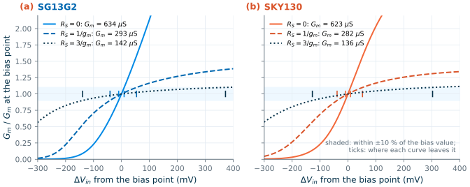
The hand calculation is a good check of Eq. (7.6). With \(R_S\) = 1.59 kΩ the simulated \(G_m\) is 293 µS in SG13G2 and 282 µS in SKY130. Using the operating-point \(g_m\) and \(g_{mb}\), Eq. (7.6) gives 298 µS and 285 µS; leaving out \(g_{mb}\) gives 315 µS and 313 µS, 8 % and 11 % too high. The body effect matters more in SKY130, which brings us to the next stage.
7.4 The source follower
Take the output from the source instead of the drain (Figure 7.5(a)) and the stage becomes a source follower: the source follows the gate, one gate–source voltage lower. It is the extreme case of degeneration, with the whole load in the source and nothing in the drain. Its gain is below one,
\[A_v = \frac{g_m}{g_m + g_{mb} + g_{ds} + G_L} \;\approx\; \frac{1}{1+\eta}, \qquad \eta = \frac{g_{mb}}{g_m}, \tag{7.7}\]where \(G_L\) is the conductance of the load (zero for the ideal current source used here). Its output resistance is low,
\[R_{out} = \frac{1}{g_m + g_{mb} + g_{ds}} \approx \frac{1}{g_m}, \tag{7.8}\]which is why followers are used as buffers: to drive a resistive or large capacitive load, or to shift a DC level, without loading the stage before them.
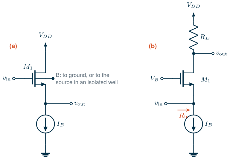
The ratio \(\eta = g_{mb}/g_m\) is where the PDKs differ. The body effect comes from the depletion charge under the channel acting as a second, weaker gate; its strength relative to the real gate scales roughly as the ratio of the depletion capacitance to the oxide capacitance [58]. The thin 2.5 nm SG13G2 oxide [15] gives the gate the upper hand, so its body effect is weaker than in SKY130 with its 4.1 nm oxide [19].
SG13G2 vs SKY130 · The body effect
With the output of the follower at 0.4 V (so \(V_{SB}\) = 0.4 V in both), the simulated \(\eta\) is 0.098 in SG13G2 and 0.153 in SKY130, and the threshold voltage has risen by 41 mV and 79 mV above its value with the bulk at the source. Eq. (7.7) then predicts follower gains of 0.886 and 0.851, which is exactly what the AC simulation gives. With the bulk tied to the source the gains rise to 0.974 and 0.980, limited only by \(g_{ds}\). Tying the bulk to the source needs an NMOS in its own isolated p-well. SG13G2 offers isolated NMOS devices built over its n-type buried layer (
nBuLay) with an n-well ring [15, 16]; the PDK models the junctions of that isolation box with itsisolboxdevice [14]. SKY130 uses a deep n-well [18]. Both cost area and add well capacitance.
Figure 7.6(a) shows the large-signal side of the follower. The output is the input shifted down by \(V_{GS}\), which is 0.35 V in SG13G2 but 0.84 V in SKY130 at this current and \(V_{SB}\). The output can therefore rise no higher than 0.80 V in SG13G2 and 0.89 V in SKY130 when the input reaches the supply. The follower spends a gate–source voltage of headroom to buy a low output resistance. The output resistances are 1.41 kΩ and 1.35 kΩ, 11 % and 15 % below \(1/g_m\) = 1.59 kΩ because of the body term in Eq. (7.8).
7.5 The common-gate stage
Now hold the gate at a fixed voltage \(V_B\) and drive the source (Figure 7.5(b)). A rise of the input reduces \(V_{GS}\) and \(V_{SB}\) together, so the drain current falls by \((g_m+g_{mb})v_{in}\) and the output rises: the gain is positive and about as large as that of a CS stage with the same load,
\[A_v \approx (g_m + g_{mb})\,(R_D \parallel r_o). \tag{7.9}\]At \(R_D\) = 10 kΩ the simulated gains are 5.95 (SG13G2) and 6.59 (SKY130). What makes the CG stage special is its input resistance. Looking into the source, the transistor absorbs a current \((g_m + g_{mb})\) per volt, so \(R_{in}\approx 1/(g_m+g_{mb})\), about 1.4 kΩ here. But this holds only when the drain sees a small load. Writing Kirchhoff’s current law at the source with \(r_o\) included gives the full result:
\[R_{in} = \frac{R_D + r_o}{1 + (g_m + g_{mb})\,r_o}. \tag{7.10}\]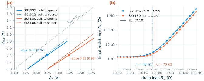
Figure 7.6(b) confirms Eq. (7.10) over six decades of \(R_D\). Below \(r_o\) (48 kΩ in SG13G2, 70 kΩ in SKY130) the input resistance is flat at 1.39 kΩ and 1.33 kΩ; at \(R_D = r_o\) it has doubled; and above that it grows in proportion to \(R_D\), divided by the intrinsic gain. With a 100 MΩ load, essentially a current source, it reaches 2.9 MΩ and 1.8 MΩ. A common-gate transistor loaded by a current source is not a low-impedance input. Remember this when we stack transistors in the next section, and again in Chapter 9, where the low input resistance is what keeps the internal node of a cascode fast.
7.6 The cascode
The cascode combines the last two stages. A common-source transistor \(M_1\) converts the input voltage into a current; a common-gate transistor \(M_2\) stacked on top passes that current to the output (Figure 7.7(a)). The physical idea is shielding: \(M_2\) holds the drain of \(M_1\) (node X) almost still, so the output voltage can swing without changing \(M_1\)’s current. A change of the output voltage must first push through \(M_2\), whose own feedback (it is a degenerated transistor, with \(r_{o1}\) as its source resistor) resists it.
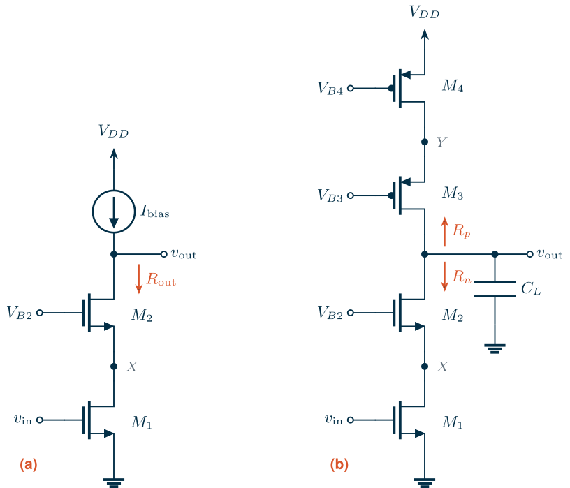
The output resistance is that of \(M_2\) degenerated by \(r_{o1}\), which by the same reasoning as Eq. (7.6) is
Key equation · Output resistance of a cascode
\[R_{out} = r_{o1} + r_{o2} + (g_{m2} + g_{mb2})\,r_{o1}r_{o2} \;\approx\; (1+\eta_2)\,\frac{g_{m2}}{g_{ds2}}\; r_{o1}. \tag{7.11}\]The cascode multiplies the output resistance of \(M_1\) by roughly the intrinsic gain of \(M_2\). With an ideal current-source load, the gain \(g_{m1}R_{out}\) becomes roughly the product of the two intrinsic gains.
The price is headroom. Both transistors must stay in saturation, so the output cannot fall below
\[V_{out,\min} = V_{DS,\mathrm{sat}1} + V_{DS,\mathrm{sat}2}, \qquad V_{DS,\mathrm{sat}} \approx \frac{2}{g_m/I_D}, \tag{7.12}\]where the approximation for the saturation voltage is exact in strong inversion and a reasonable estimate in moderate inversion [56]; in weak inversion a transistor saturates at about \(4U_T \approx 0.1\) V. At \(g_m/I_D = 15\) each device needs about 0.13 V, so the cascode needs about 0.27 V plus margin, against 0.13 V for \(M_1\) alone.
Figure 7.8 shows both effects. We stack a copy of \(M_1\) on itself, bias its gate so that node X sits at \(V_X\) = 0.25 V, and sweep the output voltage. At \(V_{DD}/2\) the output resistance rises from 48.6 kΩ to 881 kΩ in SG13G2 (×18) and from 68.1 kΩ to 1.34 MΩ in SKY130 (×20). Eq. (7.11), evaluated with the simulated small-signal values, matches both to better than 0.01 %. The gain with an ideal current-source load becomes 555 and 806, against 31 and 42 for \(M_1\) alone (Table 6.1). Below the knee, at 0.38 V in SG13G2 and 0.49 V in SKY130, \(M_2\) enters the triode region and the advantage disappears.
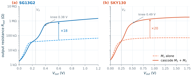
Two details deserve attention. First, the boost factor is about the same in both PDKs here because \(M_2\) is the same device as \(M_1\), which is much longer in SG13G2 (0.75 µm) than in SKY130 (0.18 µm): Chapter 6 already paid for SG13G2’s lower intrinsic gain with length. Second, \(M_1\) now works at \(V_{DS}\) = 0.25 V instead of 0.6 or 0.9 V, and its \(r_o\) drops (to 33 kΩ and 30 kΩ). Gain must always be read from the tables at the drain voltage the device will really see.
The telescopic idea
A cascode with a perfect current source above it is a fiction: the PMOS load has its own finite resistance \(R_p\), in parallel with the NMOS side’s \(R_n\). Cascoding the load as well gives the stage of Figure 7.7(b), called telescopic because the four transistors stack up like the sections of a telescope. Its gain is
\[\lvert A_v\rvert = g_{m1}\,(R_n \parallel R_p), \qquad R_n \approx (1+\eta_2)\frac{g_{m2}}{g_{ds2}}\,r_{o1}, \quad R_p \approx (1+\eta_3)\frac{g_{m3}}{g_{ds3}}\,r_{o4}. \tag{7.13}\]Writing every \(g_{ds}\) as \(g_m\) divided by the intrinsic gain \(A_i = g_m/g_{ds}\) read from the tables, and remembering that all four devices carry the same current, gives a form that needs nothing but table values:
Key equation · Gain of the telescopic stage in gm/ID terms
\[\frac{1}{\lvert A_v\rvert} = \frac{1}{(1+\eta_2)\,A_1A_2} + \frac{(g_m/I_D)_4}{(g_m/I_D)_1}\cdot\frac{1}{(1+\eta_3)\,A_3A_4}. \tag{7.14}\]
The telescopic stage reaches very high gain from one stage and four transistors, at the cost of a small output range: the output must stay at least two saturation voltages away from each rail. It is the core of the telescopic operational transconductance amplifier, a popular single-stage OTA in processes with enough supply voltage [51, 52].
7.7 Design example
We now design the telescopic stage of Figure 7.7(b) to a gain specification, in both PDKs, with the recipe of Section 6.5. This is where SG13G2’s low intrinsic gain shows most clearly.
Worked example 7.1 · A 50 dB telescopic cascode stage
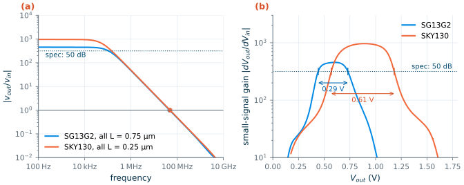
Specification. Same speed as Example 6.1 (\(f_u\) = 50 MHz into \(C_L\) = 2 pF), output biased at \(V_{DD}/2\), and a DC gain of at least 50 dB (316). We aim for 25 % margin on the prediction (395) to cover table interpolation and the body effect, which the tables (taken with \(V_{SB} = 0\)) do not include.
Steps 1–3. As in Example 6.1, \(g_{m1}\) = 628 µS; at 15 V⁻¹ the current is 41.9 µA, and the same current flows in all four devices.
Step 2, roles. \(M_1\) and the NMOS cascode \(M_2\) at 15 V⁻¹ (\(M_2\)’s transconductance sets the speed of node X). The PMOS pair \(M_3\), \(M_4\) are current-source devices: 10 V⁻¹.
Headroom. Split the supply evenly: each device gets \(V_{DS} = V_{DD}/4\), that is 0.3 V in SG13G2 and 0.45 V in SKY130. Eq. (7.12) asks for 0.13 V (NMOS) and 0.2 V (PMOS), so both splits leave margin.
Step 4, length. Use one length for all four devices and evaluate Eq. (7.14) from the tables at \(V_{DS} = V_{DD}/4\) for every tabulated L:
L (µm) 0.25 0.35 0.5 0.75 1 2 5 SG13G2, predicted gain 195 264 348 465 567 895 1576 SKY130, predicted gain 869 1813 4422 10544 13931 23202 84850 SKY130 passes at L = 0.25 µm (0.18 µm gives only 351). SG13G2 needs L = 0.75 µm, three times longer. At this length and \(V_{DS}\) = 0.3 V the SG13G2 NMOS has an intrinsic gain of only 21.8, so the NMOS half limits the gain: \((1+\eta_2)A_1A_2 = 537\), against 3445 for the PMOS half, whose intrinsic gain (43.9) is twice as high.
Step 5, widths. From the width chart: NMOS 18.18 µm (two fingers) and PMOS 24.46 µm (three fingers) in SG13G2; NMOS 6.8 µm and PMOS 10.92 µm (two fingers near the 5 µm table width) in SKY130.
Step 6, second pole. The cascode node X carries \(C_{gs2}\) plus the drain capacitance of \(M_1\), about 102 fF in SG13G2 and 16 fF in SKY130 from the tables. The pole \((g_{m2}+g_{mb2})/(2\pi C_X)\) is then at 1.1 GHz and 7.8 GHz, far above \(f_u\).
To simulate the stage we bias the three gates with ideal voltage sources whose values were found by a short operating-point run (each transistor alone, with its drain and source held at the target voltages and its gate adjusted until it carries 41.9 µA), and set the input with the DC servo of Chapter 6. Chapter 8 shows how to generate such bias voltages with current mirrors.
* Telescopic cascode stage of Worked example 7.1 (SG13G2, all L = 0.75 um, 41.9 uA)
.lib cornerMOSlv.lib mos_tt
Vdd vdd 0 1.2
Vb2 b2 0 0.6567
Vb3 b3 0 0.3177
Vb4 b4 0 0.6715
XM1 x   g  0   0   sg13_lv_nmos W=18.18u L=0.75u ng=2 m=1
XM2 out b2 x   0   sg13_lv_nmos W=18.18u L=0.75u ng=2 m=1
XM3 out b3 y   vdd sg13_lv_pmos W=24.46u L=0.75u ng=3 m=1
XM4 y   b4 vdd vdd sg13_lv_pmos W=24.46u L=0.75u ng=3 m=1
CL out 0 2p
* DC servo: holds v(out) at 0.6 V, open above ~1e-10 Hz
Vref ref 0 0.6
Vin gin 0 dc 0.336 ac 1
Eg g gin srv 0 1
Eerr e 0 out ref 1000
Rs e srv 1e9
Cs srv 0 1
.control
op
ac dec 50 100 1e11
.endc
.end
* Telescopic cascode stage of Worked example 7.1 (SKY130, all L = 0.25 um, 41.9 uA)
* Outside IIC-OSIC-TOOLS, put "set ngbehavior=hsa" in .spiceinit: without it, devices with nf > 1 are mis-binned
.lib "$PDK_ROOT/sky130A/libs.tech/ngspice/sky130.lib.spice" tt
Vdd vdd 0 1.8
Vb2 b2 0 1.2999
Vb3 b3 0 0.1979
Vb4 b4 0 0.7470
XM1 x   g  0   0   sky130_fd_pr__nfet_01v8 W=6.8   L=0.25 nf=1
XM2 out b2 x   0   sky130_fd_pr__nfet_01v8 W=6.8   L=0.25 nf=1
XM3 out b3 y   vdd sky130_fd_pr__pfet_01v8 W=10.92 L=0.25 nf=2
XM4 y   b4 vdd vdd sky130_fd_pr__pfet_01v8 W=10.92 L=0.25 nf=2
CL out 0 2p
* DC servo: holds v(out) at 0.9 V, open above ~1e-10 Hz
Vref ref 0 0.9
Vin gin 0 dc 0.765 ac 1
Eg g gin srv 0 1
Eerr e 0 out ref 1000
Rs e srv 1e9
Cs srv 0 1
.control
op
ac dec 50 100 1e11
.endc
.end
Table 7.1. Predicted and simulated performance of the telescopic stage of Worked example 7.1.
| Quantity | SG13G2 predicted | SG13G2 simulated | SKY130 predicted | SKY130 simulated |
|---|---|---|---|---|
| L (all devices) | 0.75 µm | 0.25 µm | ||
| DC gain | 465 (53.3 dB) | 455 (53.2 dB) | 869 (58.8 dB) | 966 (59.7 dB) |
| \(R_n\) / \(R_p\) | 0.87 MΩ / 5.2 MΩ | 3.8 MΩ / 2.6 MΩ | ||
| \(f_u\) | 50 MHz | 47.5 MHz | 50 MHz | 49.2 MHz |
| Phase at \(f_u\) | −92.9° | −90.4° | ||
| −3 dB bandwidth | 104 kHz | 51 kHz | ||
| Output range with gain ≥ 316 | 0.44–0.73 V | 0.57–1.18 V |
Both designs meet the specification (Figure 7.9). The predicted gains are within 2 % (SG13G2) and 11 % (SKY130) of simulation, close enough for a first pass. The phase at \(f_u\) is barely more than the −90° of the dominant pole, so the second pole is indeed far away. The unity-gain frequency of SG13G2 is 5 % low because the large PMOS cascode adds about 0.1 pF of drain capacitance to the 2 pF load. The output ranges are telling: 0.29 V of a 1.2 V supply in SG13G2, 0.61 V of 1.8 V in SKY130.
What would 60 dB take?
The course project (Section 1.6) asks for 60 dB. Running the same recipe with a target of 1000 (plus margin) picks L = 0.35 µm in SKY130; the simulated gain is 1807 (65.1 dB) with a phase of −90.7° at \(f_u\). In SG13G2 the recipe has to go to the longest tabulated length, L = 5 µm, with 110 µm wide NMOS devices. The gain is 1530 (63.7 dB), but the transit frequency of a 5 µm cascode device is only about 30 MHz, the pole at node X falls below \(f_u\), and the phase at \(f_u\) reaches −176°: as a feedback amplifier the stage would have a phase margin of 4°, which is useless (Chapter 11).
What this means for your design
In SKY130 a single telescopic stage reaches 60 dB with short, fast devices and leaves 0.6 V of swing. In SG13G2, the low intrinsic gain of the 1.2 V NMOS forces long devices, the long devices are slow, and the stacked transistors leave less than 0.3 V of swing in a 1.2 V supply. That is why the course project uses two gain stages (Chapter 12): the first stage provides gain, the second provides gain and a rail-to-rail-ish output. Where a single stage is needed in SG13G2, give the NMOS the length and the PMOS less: the PMOS half of the example had six times the output resistance it needed.
Common pitfall · Reading the tables at the wrong drain voltage
It is tempting to read the intrinsic gain at \(V_{DD}/2\), as Chapter 6 did. In a cascode every device sees only a fraction of the supply. At L = 0.75 µm the SG13G2 NMOS has an intrinsic gain of 30 at \(V_{DS}\) = 0.6 V but only 22 at 0.3 V; using the first number in Eq. (7.14) would have predicted a gain of about 870 and sent you into simulation with a design that misses by a factor of two. Always size each device at the \(V_{DS}\) (and, where it matters, the \(V_{SB}\)) it will actually have.
The 3D view of a cascode pair in layout, two gates sharing one diffusion strip, is in the PDK devices gallery; Chapter 15 explains how that sharing reduces the junction capacitance at node X.
- A resistively loaded CS stage has a gain of about \((g_m/I_D)\cdot V_{RD}\), so in a 1.2 V or 1.8 V supply it cannot exceed about 8 or 12. Active loads break this limit.
- A diode-connected load gives a gain equal to the ratio of two \(g_m/I_D\) values; a current-source load gives \(g_{m1}(r_{o1}\parallel r_{o2})\), about 27 (SG13G2) and 39 (SKY130) for Chapter 6’s transistor, but leaves the output bias undefined without feedback.
- Source degeneration divides the transconductance by \(1 + (g_m+g_{mb})R_S\) and widens the linear input range by a larger factor (26× for \(R_S = 3/g_m\)).
- The follower’s gain is about \(1/(1+\eta)\): 0.89 in SG13G2 and 0.85 in SKY130, whose body effect is stronger. It costs a \(V_{GS}\) of headroom (0.35 V and 0.84 V here).
- A common-gate input is low-impedance (\(\approx 1/g_m\)) only when its drain load is below \(r_o\).
- A cascode multiplies the output resistance by about the intrinsic gain of the cascode device, at the cost of one extra saturation voltage. A 50 dB telescopic stage needs L = 0.75 µm in SG13G2 against 0.25 µm in SKY130; 60 dB is out of practical reach in a single SG13G2 stage.
Further reading
- B. Murmann, Analysis and Design of Elementary MOS Amplifier Stages [7]: a free, careful treatment of exactly the stages in this chapter, with gm/ID design throughout.
- B. Razavi, Design of Analog CMOS Integrated Circuits, Chapter 3 [51]: the classic derivations of every single-stage amplifier, with intuition for each.
- P. G. A. Jespers and B. Murmann [56]: lookup-table design of cascodes and single-stage OTAs.
- P. R. Gray et al. [53]: the most complete small-signal analysis, including the body effect in every configuration.
- T. Chan Carusone, D. A. Johns and K. W. Martin [52]: cascode and telescopic amplifiers in the context of complete OTAs.