Chapter 15
Analog Layout
In layout, geometry becomes performance: matching, parasitics and reliability are decided by how you draw. The same schematic can work or fail depending on the polygons, so the course OTA of Chapter 12 is drawn here in both PDKs, device by device.
- Read a layout: the drawn layers of SG13G2 and SKY130, the design rules that constrain them, and the device generators that draw transistors, resistors and capacitors for you.
- Lay out a MOSFET with fingers, shared diffusions and dummies, and say what each choice does to its capacitances.
- Arrange matched devices in interdigitated and common-centroid patterns and compute what a process gradient leaves behind.
- Recognize layout-dependent effects (trench stress, well proximity) and place guard rings and taps.
- Estimate the resistance and capacitance of a route, and follow the floorplan and routing of the course OTA in both PDKs.
Contents
15.1 From schematic to polygons
A schematic says which terminals are connected; a layout says where every piece of silicon, polysilicon and metal goes. It is a set of polygons on numbered layers, stored in a GDS (or OASIS) file, and each drawn layer becomes, alone or combined with others, one of the photomasks of Chapter 17. A transistor is not a symbol in this world: it is wherever a polysilicon line crosses an active area. The overlap is the channel, its width along the poly is W, the poly width across the active area is L, and the active area on each side of the poly becomes source and drain once the implant layers have been drawn over it.
Nobody draws the dozens of rectangles of a transistor by hand. Both PDKs come with device generators (parameterized cells, PCells) that draw a legal device from its schematic parameters: IHP ships PyCells for KLayout [14, 39], and open_pdks adds device generators to Magic for SKY130 [20, 40]. Figure 15.1 shows one unit transistor of the course OTA drawn by each.
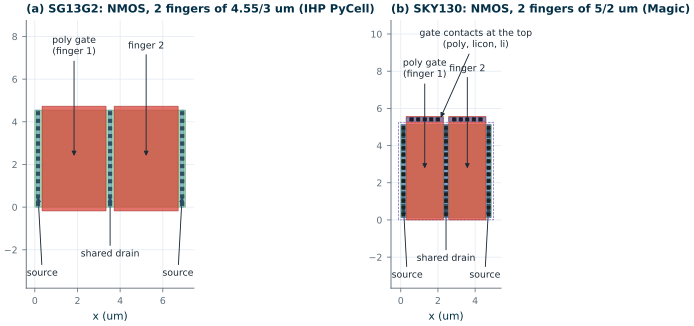
tools/layout.The figure already shows the first difference between the processes. In SG13G2, contacts land directly on the active area and Metal1 sits on top of them. In SKY130 a contact (licon) lands on the local-interconnect layer li1, a second contact (mcon) connects li1 to met1, and the generator puts the gate contacts on poly heads beyond the active area. The IHP PyCell, by contrast, leaves the gate uncontacted: the OTA layout adds a poly strap with contacts across the finger ends (Section 15.8).
15.2 Layers and design rules
Table 15.1 lists the drawn layers you meet first. Layer numbers are what the GDS file stores; KLayout’s layer properties files in each PDK give them names and colours.
Table 15.1. Main drawn layers and their GDS numbers (layer/datatype) [16, 18].
| Purpose | SG13G2 | SKY130 |
|---|---|---|
| Active area (transistor), substrate or well tap | Activ 1/0 | diff 65/20, tap 65/44 |
| Gate and poly wiring | GatPoly 5/0 | poly 66/20 |
| p+ implant (n+ is the default in SG13G2) | pSD 14/0 | psdm 94/20 (and nsdm 93/44) |
| n-well | NWell 31/0 | nwell 64/20 |
| Contact to active or poly | Cont 6/0 | licon 66/44, then li1 67/20 and mcon 67/44 |
| First metal, first via | Metal1 8/0, Via1 19/0 | met1 68/20, via 68/44 |
| Further metals | Metal2–5: 10, 30, 50, 67; TopMetal1/2: 126, 134 | met2–met5: 69, 70, 71, 72 (datatype 20) |
| Resistor and capacitor markers | PolyRes 128/0, SalBlock 28/0, MIM 36/0 | poly-resistor id 66/13, rpm 86/20, capm 89/44 |
Design rules are the geometric limits of the process steps: minimum widths and spacings, enclosures of one layer by another, extensions of poly beyond active, and many conditional rules for wide or long shapes. Table 15.2 gives a handful; the SG13G2 layout-rules document and the SkyWater periphery rules list several hundred each.
Table 15.2. A few minimum design rules (µm), read from the PDK files: SG13G2 from the PyCell library's sg13g2_tech_mod.json, SKY130 from the KLayout rule deck sky130A_mr.drc [16, 18].
| Rule | SG13G2 | SKY130 |
|---|---|---|
| Active width / spacing | 0.15 / 0.21 | 0.15 / 0.27 |
| Poly (gate) width / spacing | 0.13 / 0.18 | 0.15 / 0.21 |
| Contact size / spacing | 0.16 / 0.18 | licon 0.17 / 0.17 |
| Local interconnect width / spacing | — | 0.17 / 0.17 |
| Metal1 width / spacing | 0.16 / 0.18 | 0.14 / 0.14 |
| Via1 size / spacing | 0.19 / 0.22 | 0.15 / 0.17 |
| Metal2 width / spacing | 0.20 / 0.21 | 0.14 / 0.14 |
| n-well width / spacing | 0.62 / 0.62 | 0.84 / 1.27 |
Most rules are minimums, and an analog layout rarely needs them: a current mirror at L = 2 µm is nowhere near the minimum poly width. The rules that bite in analog work are the ones about large shapes (wide-metal spacing, slots, density), about devices (gate extension, contact-to-gate spacing, resistor and capacitor rules) and about wells (spacing between wells at different potentials). The DRC of Chapter 16 checks all of them; you do not have to remember them.
15.3 Laying out a MOSFET
A wide transistor is never drawn as one long gate. It is split into fingers, parallel gates of width \(W_f = W/n_f\) that share their source and drain diffusions with their neighbours. Fingers do three things:
- They make the device compact. An 80 µm wide transistor becomes a block of about 20 × 4 µm instead of a sliver 80 µm long.
- They cut the drain capacitance. With an even number of fingers the drain diffusions are all inner ones, each shared by two gates, so the drain junction is about half as large as for a single finger. For the output transistor \(M_6\) of the course OTA the simulated drain junction capacitance at mid-supply falls from 23.4 fF as one finger to 12.8 fF as the 24 fingers of the layout (SG13G2), and from 23.4 to 14.2 fF as 12 fingers (SKY130).
- They cut the gate resistance. The poly of a finger is a resistor from its contact to its far end; a long finger with one contact can add a pole near the device’s \(f_T\). Keep fingers short and contact them, or strap them, at one or both ends.
There is a limit: Chapter 6 showed that the models (especially SKY130’s binned ones) change with finger width. Keep every finger at the width the gm/ID tables were built with and reach large widths with more fingers or more units. That is why every unit of the course OTA is 4.5 to 10 µm wide per finger.
The ends of a row are different from its middle: the outermost fingers see a different etch environment and a different stress from the trench next to them (Section 15.5). Dummy devices, extra gates at each end of a row with all terminals on a rail, make every active finger see the same neighbours. They cost area and a little capacitance on the rail, and every matched row in the course OTA has one at each end.
15.4 Matching techniques
Two transistors that should be identical differ for two reasons. Random mismatch, the Pelgrom term of Chapter 13, falls only with area; layout cannot reduce it beyond making the devices larger [75]. Systematic mismatch comes from gradients across the die (of oxide thickness, doping, temperature or stress) and from differences in the devices’ surroundings. Layout can cancel most of it [60]:
- Unit devices. Build every matched device, and every ratio, from copies of one unit, as Chapter 8 did for the mirror ratios. Two units of 9.1 µm match far better than one device of 18.2 µm and another of 9.1 µm.
- Same orientation and same surroundings. Every unit points the same way (the current flows in the same direction), sits in a row with the same neighbours, and has a dummy at each row end.
- Common centroid. Arrange the units so that the centroids (the centres of gravity) of the matched devices coincide. Then a gradient that is linear across the array affects each device by the same average amount.
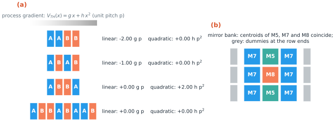
Figure 15.2(a) works this out for a process parameter that varies along a row, \(V_{TH}(x) = g\,x + h\,x^2\), with the units of devices A and B at unit pitch \(p\). The difference of their average thresholds is
\[\Delta V_{TH} = \overline{V_{TH}}_A - \overline{V_{TH}}_B. \tag{15.1}\]Side by side (AABB), a linear gradient gives \(\Delta V_{TH} = 2gp\); interleaving (ABAB) halves it; the common-centroid row ABBA cancels it completely, but a quadratic gradient now leaves \(2hp^2\). The eight-unit pattern ABBA·BAAB cancels both. The 3 × 3 array of panel (b) is the two-dimensional version: the centroids of \(M_5\), \(M_7\) and \(M_8\), the three devices that share the bias of the course OTA, all sit at the centre of the array.
Worked example 15.1 · When does a gradient matter for the input pair?
The SG13G2 input-pair units are 7 µm wide plus a 1 µm gap, so \(p\) = 8 µm, and the pair’s random offset is σ = 1.6 mV (Lab 7). Side by side (AABB) a linear gradient \(g\) leaves \(\Delta V_{TH} = 2gp\); it equals the random σ when \(g = \sigma/(2p)\) = 1.6 mV/16 µm = 0.1 mV/µm, or 100 mV per millimetre. Interleaved (ABAB) the gradient would have to be twice as steep, and the ABBA row of the layout cancels it to first order whatever its size; a quadratic term then leaves \(2hp^2\).
The same arithmetic explains where common centroids matter most. The four units of this pair span 32 µm, so a gradient has little distance to act over. A capacitor array of Chapter 21, spread over a few hundred micrometres, collects ten times the gradient for each unit of distance between its matched elements, while its random mismatch per element does not grow. The arrangement costs nothing in area: the same units are only placed differently, and the routing gets slightly longer.
What this means for your design
Match by construction, in this order: the same unit, the same orientation, the same neighbours, the same centroid. Then route the matched devices symmetrically, so that their wires see the same resistance and the same coupling, and keep unrelated metal out of the area above them. None of this reduces random mismatch; only area does. Spend the area where Chapter 13 says the offset comes from: the input pair, and in SKY130 the PMOS mirror.
15.5 Layout-dependent effects and guard rings
A transistor’s current depends not only on W and L but on what is drawn around it [84]. The two effects that matter most at 130 nm are:
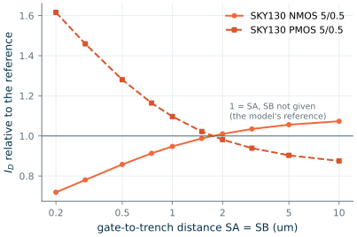
- Trench stress (length of diffusion, LOD). The oxide in the shallow trench of Chapter 17 squeezes the silicon next to it and changes the mobility. The model describes it with the distances SA and SB from the gate to the trench edge on either side [83]. Stress raises the hole mobility and lowers the electron mobility, so PMOS and NMOS move in opposite directions.
- Well proximity (WPE). Ions of the well implant scatter off the edge of the resist mask into the silicon next to it, so a transistor close to a well edge gets a higher threshold [84].
Figure 15.3 shows the size of the first effect in the SKY130 models, which take SA and SB as instance parameters. At the 50 µA bias of Chapter 4, an NMOS whose trench edge is 0.2 µm from the gate carries 28 % less current than the model’s reference, and a PMOS 62 % more; at 10 µm the NMOS has 7 % more and the PMOS 13 % less. The SG13G2 MOSFET subcircuits have no SA or SB parameters, so their models do not show the effect, although the silicon certainly has it.
You cannot remove these effects; you can make matched devices see the same amount of them. Units of the same size, in rows, with dummies at the ends, have the same SA and SB for corresponding fingers. Matched devices at the same distance from the well edge, and as far from it as the area allows, have the same well proximity. This is why the PMOS mirror of the course OTA sits in the middle of its n-well with a dummy at each end.
Common pitfall · Trusting the post-layout netlist to include layout effects
Neither the Magic extraction of Chapter 16 nor the KLayout LVS netlists write SA, SB or well-proximity parameters for these PDKs. The post-layout simulation therefore shows the effect of every wire’s capacitance but none of the stress. A design that relies on the post-layout simulation to catch a mirror whose reference device sits at the end of a row and whose output device sits in the middle will not see the error. Draw matched devices so that the effects cancel, and do not expect a simulation to tell you when they do not.
Guard rings and taps. The p-substrate and every n-well must be tied to their supplies through taps, close to the transistors: the substrate under an NMOS that carries current must not drift, and in a CMOS process a well that is poorly tapped invites latch-up, in which the parasitic bipolar transistors of the n-well and the substrate turn each other on and short the supply. A ring of substrate taps around a group of NMOS devices (a p+ guard ring tied to ground) and a ring of n+ taps inside each n-well (tied to \(V_{DD}\)) keep the potentials fixed and collect carriers injected by neighbouring circuits [60]. The course OTA has a p+ ring around each NMOS group and an n+ ring in its n-well (Figure 15.4). For blocks that must be quiet, such as a reference next to a digital block, add a second ring and keep the noisy circuit’s substrate current away.
15.6 Resistors and capacitors
Resistors are strips of polysilicon. The silicide that makes poly a good conductor (7 Ω/sq for SG13G2’s rsil) is blocked over the body of a precision resistor, which leaves the doped poly’s own sheet resistance: 260 Ω/sq for SG13G2’s p+ poly resistor rppd and 1360 Ω/sq for its high-resistance rhigh, and 319.8 Ω/sq for SKY130’s res_high_po [14, 20]. The resistance of a strip of length \(l\) and width \(w\) is
where \(R_{end}\) is the resistance of each contacted head. Wider resistors match better and their resistance depends less on the etch of their edges; keep them away from the minimum width. The nulling resistor \(R_z\) of the course OTA is an rppd strip of 1 × 7.82 µm in SG13G2 (2.10 kΩ) and a res_high_po_0p69 strip of 0.69 × 4.49 µm in SKY130, each drawn by the PDK’s generator from the value of Chapter 12.
Capacitors for analog use are metal-insulator-metal (MIM) capacitors: a thin dielectric between a lower metal and an extra top plate. SG13G2’s cap_cmim sits between Metal5 and TopMetal1 at about 1.5 fF/µm², SKY130’s cap_mim_m3_1 between met3 and a capm plate under met4 at about 2.0 fF/µm² (Chapter 17). The 1 pF Miller capacitor of the OTA is a square of 25.8 µm (SG13G2) or 22.2 µm (SKY130) on a side, about a tenth of the block’s area. Two practical rules:
- Connect the bottom plate to the low-impedance node. The bottom plate couples to the substrate and to everything below it; on the output node, which is driven hard, that parasitic does no harm. In the course OTA the bottom plate is connected to
outand the top plate to \(R_z\). - Keep the plates’ surroundings symmetric for matched capacitors, and build ratios from unit capacitors, exactly as for transistors.
15.7 Routing and parasitics
Every wire is a resistor and a capacitor. Table 15.3 gives the nominal values the PDKs’ Magic extraction rules use.
Table 15.3. Wiring resistance and capacitance to the substrate, from the extraction rules of each PDK's Magic technology file (nominal values) [40, 20]. Fringe and coupling capacitances come on top of the area values.
| Layer | SG13G2 R□ (mΩ/sq) | SG13G2 Carea (aF/µm²) | SKY130 R□ (mΩ/sq) | SKY130 Carea (aF/µm²) |
|---|---|---|---|---|
| Local interconnect | — | — | 12 800 | 37.0 |
| Metal1 | 110 | 35.0 | 125 | 25.8 |
| Metal2 | 88 | 18.2 | 125 | 17.5 |
| Metal3 | 88 | 12.0 | 47 | 12.4 |
| Metal4 | 88 | 8.9 | 47 | 8.4 |
| Top metal | 18 (TopMetal1), 11 (TopMetal2) | 5.6, 3.2 | 29 (met5) | 6.3 |
| Via (one cut) | 9 Ω (Via1–4) | 4.5 Ω (via), 3.4 Ω (via2, via3) |
Worked example 15.2 · The wire to the gate of M6
Take a route of 60 µm of 0.5 µm wide Metal2 for the first-stage output \(x_1\), from the input pair to the gate of \(M_6\) (the order of magnitude of the routes in Figure 15.4). In SG13G2 that is 120 squares × 88 mΩ = 10.6 Ω and an area capacitance of 30 µm² × 18.2 aF/µm² = 0.55 fF, plus a few femtofarads of fringe and coupling. Compared with the node’s own capacitance, the gate of \(M_6\) (about 0.3 pF, \(C_1\) of Chapter 11), the wire is negligible, and its resistance against the output resistance of the first stage (hundreds of kilohms) more so. In a small analog block the devices dominate the parasitics; the wires matter where they are long, wide or close to a sensitive node. The extraction of Chapter 16 confirms it: the 36 wiring capacitors of the SG13G2 OTA add up to 169 fF, the largest being 70 fF on the tail node and 35 fF on the output.
The resistance of a wire matters where currents are large or nodes are low-impedance: supply rails, the source of a large transistor, the ground of a current mirror. A current mirror whose two sources are connected by a 20 Ω rail carrying 60 µA has a 1.2 mV difference in \(V_{GS}\), which at \(g_m/I_D\) = 8 is a 1 % error. Give each matched device its own path to the rail, or make the rail wide.
15.8 The course OTA in both PDKs
Figure 15.4 shows the two-stage OTA of Chapter 12 laid out in both PDKs, with every technique of this chapter.
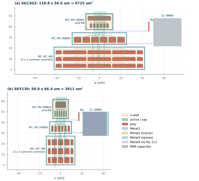
tools/layout/ota_layout.py, both at the same scale: (a) SG13G2, (b) SKY130. Dotted boxes: the three device groups, each in its guard ring. Metal2 tracks run over each row, one Metal3 spine per net runs vertically, and Metal4 connects Rz and Cc.Table 15.4. Floorplan of the course OTA. Units are generator cells; dummies in brackets.
| Group | Devices and arrangement | SG13G2 unit | SKY130 unit |
|---|---|---|---|
| NMOS mirror bank | M8 (1 unit), M5 (2), M7 (6) as a 3 × 3 common centroid, (6 dummies) | 11.28/5 µm, 4 fingers | 10/2 µm, 2 fingers |
| Input pair | M1, M2 (2 units each) as ABBA, (2 dummies) | 9.1/3 µm, 2 fingers | 5/1.5 µm, 1 finger |
| PMOS mirror | M3, M4 (2 units each) as ABBA, (2 dummies) | 6.66/0.5 µm, 2 fingers | 5/0.5 µm, 1 finger |
| Second stage | M6, one device | 79.92/0.5 µm, 24 fingers | 60/0.5 µm, 12 fingers |
| Passives | Rz, Cc | rppd 1 × 7.82 µm, cmim 25.8² µm² | res_high_po 0.69 × 4.49 µm, MIM 22.2² µm² |
| Size | 118.8 × 56.6 µm = 6725 µm² | 58.9 × 66.4 µm = 3911 µm² |
Floorplan. The devices form three groups stacked from the ground side up: the NMOS mirror bank, the input pair, and the PMOS devices in one n-well. Each group has its own guard ring. The passives sit to the right, where the long Metal4 routes to them do not cross any matched device. The input pair is in the middle, between the bias bank and the load it drives, so that its two halves see the same neighbours.
Routing. Every row has a set of horizontal Metal2 tracks, one per net it uses; every net has one vertical Metal3 spine, and the spines run through the middle of all three groups. The order of the spines keeps the two inputs and the two first-stage nodes next to each other, so that their couplings to the surrounding nets are similar. Pins for inp, inn, out, vdd, vss and ibias are Metal3 labels at the ends of the spines.
How it is made. None of the devices is drawn by the script. tools/layout/gen_cells_sg13g2.py runs the IHP PyCells in KLayout and tools/layout/gen_cells_sky130.tcl runs Magic’s generators, one cell per unit. tools/layout/ota_layout.py then places the cells, adds the gate straps and guard rings, routes the nets on the grid and writes a flat GDS file. It uses only KLayout’s Python module, so it runs in IIC-OSIC-TOOLS or anywhere pip install klayout works:
cd /foss/designs/art_of_aicd
klayout -b -r tools/layout/gen_cells_sg13g2.py -rd out=tools/layout/sg13g2/cells.gds
CELLS_OUT=tools/layout/sky130/cells magic -dnull -noconsole \
    -rcfile $PDK_ROOT/sky130A/libs.tech/magic/sky130A.magicrc tools/layout/gen_cells_sky130.tcl
python3 tools/layout/ota_layout.py sg13g2 sky130      # -> tools/layout/<pdk>/ota2s.gds
klayout tools/layout/sg13g2/ota2s.gds &              # look at it
Tools. KLayout [39] is the viewer and editor of the SG13G2 flow, with the PDK’s PyCells, DRC and LVS; its Python and Ruby interfaces script everything above. Magic [40] is the traditional SKY130 editor, with interactive DRC as you draw, the device generators and parasitic extraction. Both read and write GDS, so you can draw in one and check in the other. For larger generated layouts, gLayout [44, 5] builds analog cells (mirrors, pairs, whole OTAs) from Python with routing and matching patterns built in. The script of this chapter is the do-it-yourself version of the same idea, small enough to read in an afternoon. Whatever you use, Chapter 16 is the next step: proving that the polygons are legal and that they are the circuit of Chapter 12.
SG13G2 vs SKY130 · Same circuit, 1.7 times the area
The SG13G2 OTA needs 72 % more area for the same specification because of decisions taken in Chapters 6 and 12: its low intrinsic gain forced a 3 µm input pair and long, wide current sources (5 µm), while SKY130 reached the gain with 1.5 µm and 2 µm. The routing is the same in both, and so is the MIM capacitor, which takes about a tenth of either block. The technology’s minimum rules (Table 15.2) do not enter: a circuit like this is sized by its electrical specification, not by its smallest feature.
Try it · Lab 8
Lab 8 regenerates these layouts, opens them in KLayout and Magic, and takes them through DRC, LVS, extraction and post-layout simulation (Chapter 16). Generate the input pair as AABB (
ota_layout.py <pdk> --pair=AABB --out=/tmp/aabb) and check that DRC and LVS still pass: the circuit is the same, only its sensitivity to gradients has changed.
- A layout is polygons on layers; a transistor is poly crossing active. Use the PDK’s device generators (IHP PyCells in KLayout, Magic’s generators for SKY130) and add only what a designer adds: placement, straps, rings and routing.
- Split wide transistors into fingers at the width the gm/ID tables were built with. Fingers halve the drain capacitance (23.4 → 12.8 fF for the SG13G2 output device) and shorten the gates. Put a dummy at each end of a matched row.
- Build matched devices from units in the same orientation with the same neighbours, and give them a common centroid: ABBA cancels a linear gradient, ABBA·BAAB a quadratic one too. Only area reduces random mismatch.
- Trench stress changes a SKY130 transistor’s current by tens of per cent (−28 % NMOS, +62 % PMOS at 0.2 µm), and post-layout netlists do not include it. Make matched devices see the same surroundings; tie substrate and wells with guard rings.
- Wires are small resistors and capacitors next to the devices in a block like this (169 fF in total for the SG13G2 OTA); they matter on supply rails, long routes and sensitive nodes. The course OTA takes 6725 µm² in SG13G2 and 3911 µm² in SKY130.
Further reading
- A. Hastings, The Art of Analog Layout [60]: the standard reference for everything in this chapter, from fingers and dummies to guard rings, resistors and capacitors.
- P. G. Drennan, M. L. Kniffin and D. R. Locascio [84]: how well proximity and trench stress affect analog circuits, with measurements.
- M. J. M. Pelgrom et al. [75]: random mismatch, and why only area helps against it.
- The IHP SG13G2 layout rules [16] and the SkyWater periphery rules [18]: read the device and resistor sections before you draw.