Chapter 6
The gm/ID Design Methodology
Instead of trusting an equation that no longer fits modern transistors, gm/ID design reads the transistor's real behaviour from simulated tables and sizes every device from three choices: gm/ID, L and current.
- Explain why the square law is a poor guide for sizing transistors in a 130 nm process.
- Define gm/ID, relate it to the inversion level, and read the four gm/ID design charts.
- Build gm/ID lookup tables for SG13G2 and SKY130 with ngspice and query them in Python.
- Size a transistor and a common-source stage with a seven-step recipe, and check the result by simulation.
- Choose the channel length from gain, speed and area requirements.
Contents
6.1 Why the square law fails for sizing
The classic way to size a MOSFET goes like this. Pick an overdrive voltage \(V_{OV} = V_{GS} - V_{TH}\), say 200 mV. Use the square law from Chapter 4,
\[I_D = \tfrac{1}{2}\mu_n C_{ox}\frac{W}{L}V_{OV}^2, \qquad g_m = \frac{2I_D}{V_{OV}}, \tag{6.1}\]to turn the required current and transconductance into \(W/L\). Then simulate, discover that the circuit is 30 % off, adjust, and repeat. The square law [71, 51] is a wonderful tool for building intuition, but as a sizing tool it has three problems in a 130 nm process.
- \(V_{TH}\) is not a sharp boundary. Current does not switch on at threshold. It grows exponentially below it and only gradually turns into the square law above it. The region in between, moderate inversion, is exactly where most low-power analog circuits are biased today.
- Short-channel devices are not square-law devices. Velocity saturation and mobility degradation flatten the current at high overdrive (Section 4.6), and the effective \(\mu_n C_{ox}\) changes with bias, length and even width.
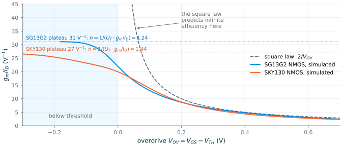
- The square law predicts impossible efficiency. Dividing the two halves of Eq. (6.1) gives \(g_m/I_D = 2/V_{OV}\), which grows without bound as \(V_{OV} \to 0\). A real transistor cannot do that.
Figure 6.1 shows the third problem directly. It compares \(2/V_{OV}\) with the \(g_m/I_D\) that ngspice computes from the PDK models of an NMOS transistor with L = 0.5 µm in each process. Above about 150 mV of overdrive the square law is within 25 % of the truth (above 158 mV for SG13G2 and 142 mV for SKY130). Below it the real curve bends over and settles at a plateau of 31 V⁻¹ in SG13G2 and 27 V⁻¹ in SKY130, while the square law heads off to infinity.
The way out was proposed by Silveira, Flandre and Jespers in 1996 [74] and developed into a complete method by Jespers and Murmann [57, 56]: stop fitting equations to the transistor, and use the transistor itself. Simulate one device once, over every bias and length you might use, store the results in a table, and size every transistor in the design by looking it up. The design variable that makes this work is \(g_m/I_D\).
6.2 gm/ID and the inversion level
The transconductance efficiency of a transistor is the transconductance it delivers per unit of bias current:
\[\frac{g_m}{I_D} = \frac{1}{I_D}\frac{\partial I_D}{\partial V_{GS}} = \frac{\partial \ln I_D}{\partial V_{GS}}. \tag{6.2}\]It has units of V⁻¹. A transistor at \(g_m/I_D = 15\ \mathrm{V^{-1}}\) biased at 10 µA gives 150 µS of transconductance. Because transconductance is what amplifies and current is what costs power, \(g_m/I_D\) is the exchange rate between the two.
The two limits of Eq. (6.2) are easy to evaluate.
- In weak inversion, below threshold, the drain current is a diffusion current that grows exponentially with gate voltage, \(I_D \propto \exp\!\big(V_{GS}/(nU_T)\big)\). Here \(U_T = kT/q \approx 25.9\) mV at 27 °C, and \(n \approx 1.2\)–1.5 is the slope factor, set by how well the gate controls the channel surface potential. Then \(g_m/I_D = 1/(nU_T)\), a constant of about 25 to 32 V⁻¹. This is the highest efficiency a MOSFET can reach.
- In strong inversion, well above threshold, the square law applies and \(g_m/I_D = 2/V_{OV}\), which falls as the device is driven harder.
The EKV model [72, 59] joins the two regions with a single expression in terms of the inversion coefficient \(IC\), the drain current normalized to a technology current that scales with \(W/L\):
Key equation · gm/ID and the inversion coefficient
\[\frac{g_m}{I_D} = \frac{1}{nU_T}\cdot\frac{2}{1+\sqrt{1+4\,IC}}, \qquad IC = \frac{I_D}{I_\mathrm{spec}}, \qquad I_\mathrm{spec} = 2n\mu C_{ox}\frac{W}{L}U_T^2. \tag{6.3}\]\(IC < 0.1\) is weak inversion, \(0.1 < IC < 10\) moderate inversion and \(IC > 10\) strong inversion. With \(n = 1.3\) these boundaries sit at \(g_m/I_D \approx 27\) and \(8\ \mathrm{V^{-1}}\).
You will rarely evaluate Eq. (6.3) numerically, because the tables in Section 6.4 replace it. Its value is the picture it gives: \(g_m/I_D\) is a direct measure of the inversion level, from about 30 V⁻¹ deep in weak inversion down to 3 or 4 V⁻¹ when the transistor is driven hard.
It also shows the property that makes the method practical. \(IC\) depends on \(I_D\) only through \(I_D/(W/L)\), so for a fixed length \(g_m/I_D\) depends on the current density \(I_D/W\), not on \(W\) itself. Characterize one width, and the results apply to every width: double \(W\) and \(I_D\) together and \(g_m/I_D\), \(V_{GS}\) and the transit frequency stay the same, while \(g_m\) and every capacitance double. (Section 6.6 shows where this scaling breaks.)
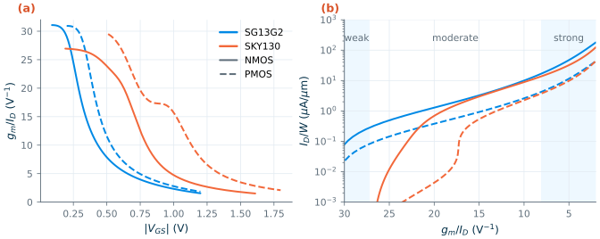
Figure 6.2 shows both views of the inversion level for NMOS and PMOS transistors with L = 0.5 µm. In panel (a), \(g_m/I_D\) falls from its plateau to about 3 V⁻¹ as \(\lvert V_{GS}\rvert\) rises. The curves of the two PDKs are shifted by their threshold voltages. At this length the SG13G2 NMOS turns on at about 0.27 V and the SKY130 NMOS at 0.63 V; the PMOS thresholds are 0.37 V and 0.98 V. Panel (b) plots the current density against \(g_m/I_D\). The two NMOS curves almost coincide in moderate inversion: at \(g_m/I_D = 15\ \mathrm{V^{-1}}\) the SG13G2 device carries 3.3 µA per micrometre of width and the SKY130 device 3.0 µA/µm.
What this means for your design
Think of \(g_m/I_D\) as a dial with three settings. High (18–25 V⁻¹, weak to moderate inversion): the most transconductance for your current, so the lowest power and noise for a given \(g_m\), but wide, slow devices. Medium (10–18 V⁻¹, moderate inversion): the usual choice for amplifying transistors. Low (5–10 V⁻¹, strong inversion): compact, fast devices with a larger \(V_{OV}\), which also makes them less sensitive to threshold mismatch. That is why current mirrors and tail sources live here.
6.3 The four charts
Everything you need to size a transistor can be read from four curves, all plotted against \(g_m/I_D\) (or \(V_{GS}\)) for a few channel lengths:
| Chart | Plots | Tells you |
|---|---|---|
| Bias | \(g_m/I_D\) vs \(V_{GS}\) | the gate voltage, and so the headroom, at a chosen inversion level |
| Width | \(I_D/W\) vs \(g_m/I_D\) | the width needed to carry the bias current |
| Speed | \(f_T\) vs \(g_m/I_D\) | the transit frequency, \(f_T = g_m/(2\pi C_{gg})\), the frequency at which the device’s current gain falls to one |
| Gain | \(g_m/g_{ds}\) vs \(g_m/I_D\) | the intrinsic gain, the largest voltage gain one transistor can give |
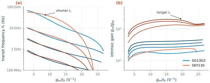
We have met the first two in Figure 6.2. Figure 6.3 shows the speed and gain charts for four lengths in each PDK.
Three trends hold in both processes.
- Speed falls as \(g_m/I_D\) rises. A device in weak inversion needs a large width to carry its current, and the extra gate capacitance slows it down. At \(g_m/I_D = 15\ \mathrm{V^{-1}}\), a minimum-length NMOS reaches \(f_T \approx 9.8\) GHz in SG13G2 and 16 GHz in SKY130; at L = 2 µm both are below 200 MHz.
- Speed falls steeply with length. In long devices \(f_T\) scales roughly as \(1/L^2\) (the current falls as \(1/L\) and the gate capacitance rises as \(L\)). Doubling L from 1 to 2 µm cuts \(f_T\) by a factor of 3.7 in SG13G2.
- Gain rises with length, because a longer channel is less affected by the drain voltage, so \(g_{ds}\) falls.
The fourth observation is a difference between the processes, and it is large.
SG13G2 vs SKY130 · Intrinsic gain
At \(g_m/I_D = 15\ \mathrm{V^{-1}}\) and L = 0.5 µm, the SKY130 NMOS has an intrinsic gain of 130, five times the 26 of the SG13G2 NMOS. Even at L = 2 µm, SG13G2 reaches only 41 against 202 for SKY130. The SG13G2 core transistor is a 1.2 V device built for logic speed: its gate oxide is about 2.5 nm thick (targets of 2.45 and 2.65 nm) [15], against 4.1 nm for the SKY130 1.8 V device [19]. Its threshold also rises strongly at short lengths (Chapter 4), a sign of heavy halo implants, which are known to raise the output conductance of longer devices. Expect to use longer channels, cascodes or more gain stages in SG13G2 than in SKY130 for the same gain. The SG13G2 thick-oxide 3.3 V devices behave differently again.
A figure of merit for speed and power
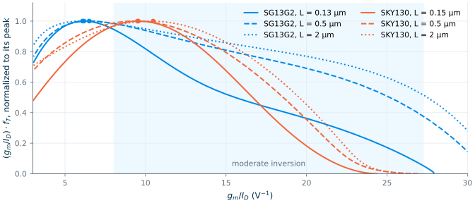
If both speed and power matter, a useful single number is the product \((g_m/I_D)\cdot f_T\): transconductance per unit current, times speed. Figure 6.4 shows that this product peaks in moderate inversion, close to the strong-inversion boundary: at \(g_m/I_D \approx 6\) V⁻¹ in SG13G2 and \(\approx 10\) V⁻¹ in SKY130, for every length shown. Biasing deeper in strong inversion buys little extra speed for a lot of extra current; biasing deeper in weak inversion saves current but loses speed quickly. This is why many wideband designs start at a \(g_m/I_D\) of 8 to 12 V⁻¹, and low-power designs at 15 to 20 V⁻¹.
The demo below puts the four charts of both PDKs side by side. Pick a chart, a length and a \(g_m/I_D\), and it sizes the input transistor of the course OTA from the same tables.
6.4 Building lookup tables
A lookup table is the four charts in numerical form: every small-signal quantity of a transistor, stored on a grid of \((L, V_{DS}, V_{GS})\). Building one is a single ngspice run. Figure 6.5 shows the testbench: one transistor of fixed width (we use W = 5 µm) with ideal sources on its gate and drain, source and bulk grounded.
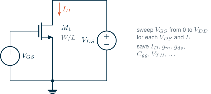
For this course the tables cover 11 lengths from Lmin to 5 µm, 10 or 11 drain voltages, and gate voltages from 0 to VDD in 10 mV steps, for both NMOS and PMOS in both PDKs. All eleven lengths are simulated at once, as eleven transistors in parallel between the same gate and drain sources. On a laptop the four tables take about five seconds to build. The script is tools/gmid/techsweep.py, and the tables it writes are in tools/data/.
The core of the testbench is the list of operating-point values to save. Their names differ between the PDKs, because SG13G2 uses the PSP compact model, compiled from Verilog-A and loaded into ngspice through OSDI, while SKY130 uses BSIM4, which is built into ngspice (Chapter 3):
* gm/ID characterization of sg13_lv_nmos, one length (IIC-OSIC-TOOLS loads the PSP .osdi via .spiceinit)
.lib cornerMOSlv.lib mos_tt
Vds d 0 0.6
Vgs g 0 0
XM1 d g 0 0 sg13_lv_nmos W=5u L=0.5u ng=1 m=1
* PSP device inside the subcircuit: n.<instance>.<model>; overlap caps are cgsol and cgdol
.save @n.xm1.nsg13_lv_nmos[ids] @n.xm1.nsg13_lv_nmos[gm] @n.xm1.nsg13_lv_nmos[gds]
+     @n.xm1.nsg13_lv_nmos[vth] @n.xm1.nsg13_lv_nmos[cgg]
+     @n.xm1.nsg13_lv_nmos[cgsol] @n.xm1.nsg13_lv_nmos[cgdol]
.control
dc vgs 0 1.2 0.01
wrdata sg13_lv_nmos_L0p5.txt @n.xm1.nsg13_lv_nmos[ids] @n.xm1.nsg13_lv_nmos[gm] @n.xm1.nsg13_lv_nmos[gds]
.endc
.end
* gm/ID characterization of nfet_01v8, one length (W and L in um: the library sets .option scale=1u)
.lib "$PDK_ROOT/sky130A/libs.tech/ngspice/sky130.lib.spice" tt
Vds d 0 0.9
Vgs g 0 0
XM1 d g 0 0 sky130_fd_pr__nfet_01v8 W=5 L=0.5 nf=1 ad=1.45 as=1.45 pd=10.58 ps=10.58
* BSIM4 device inside the subcircuit: m.<instance>.m<model>; overlap caps are cgso and cgdo
.save @m.xm1.msky130_fd_pr__nfet_01v8[id] @m.xm1.msky130_fd_pr__nfet_01v8[gm]
+     @m.xm1.msky130_fd_pr__nfet_01v8[gds] @m.xm1.msky130_fd_pr__nfet_01v8[vth]
+     @m.xm1.msky130_fd_pr__nfet_01v8[cgg] @m.xm1.msky130_fd_pr__nfet_01v8[cgso]
+     @m.xm1.msky130_fd_pr__nfet_01v8[cgdo]
.control
dc vgs 0 1.8 0.01
wrdata nfet_01v8_L0p5.txt @m.xm1.msky130_fd_pr__nfet_01v8[id] @m.xm1.msky130_fd_pr__nfet_01v8[gm]
.endc
.end
Common pitfall · Leaving out the overlap capacitance
Both models report the gate-to-source and gate-to-drain overlap capacitances separately from the intrinsic gate capacitance
cgg. The true total gate capacitance is \(C_{gg} =\)cgg+cgsol+cgdolin SG13G2 andcgg+cgso+cgdoin SKY130. We checked both sums against an AC simulation of the gate current, and they agree to within 0.1 %. The overlap is not a detail: for a minimum-size SG13G2 NMOS at mid-supply it is 77 % of the total (1.24 fF of 1.60 fF). Forget it and your \(f_T\) will be four times too optimistic.
With the tables in hand, sizing is a function call. The helper in tools/aicd/lookup.py interpolates the tables in \(L\) and \(V_{DS}\) and inverts them in \(g_m/I_D\):
from aicd.lookup import Device

n = Device("sg13g2", "n")                     # or Device("sky130", "p"), ...
s = n.size(gm_id=15, L=0.75, VDS=0.6, ID=41.9e-6)
print(f"W = {s['W']:.2f} um, VGS = {s['VGS']:.3f} V, gm/gds = {s['gm_gds']:.1f}, fT = {s['ft']/1e9:.2f} GHz")
# W = 18.05 um, VGS = 0.325 V, gm/gds = 30.1, fT = 1.10 GHz
You do not have to use our scripts. Murmann’s open-source starter kit [46] comes with ready-made tables for SKY130 and SG13G2, and the pygmid package [45] reads them in Python. That is the route taken by the JKU course [2]; the IHP Analog Academy uses a similar sweep [3]. Building your own once is still worth it, because you then know exactly what is in the table.
Try it · Lab 2
Lab 2 builds the testbench of Figure 6.5 in Xschem, sweeps it in ngspice and plots the four charts for your chosen PDK. Then change the corner to
mos_ss/ssand see which charts move.
6.5 A sizing recipe
With the tables available, every transistor in a design is sized by the same seven steps.
- Find the transconductance the device must provide. For a stage driving a capacitive load \(C_L\) with a unity-gain frequency \(f_u\), \(g_m = 2\pi f_u C_L\). Other specifications (noise, gain) lead to \(g_m\) in the same way.
- Choose \(g_m/I_D\) for the device’s role, using the dial of Section 6.2: 12 to 20 V⁻¹ for amplifying devices, 5 to 10 V⁻¹ for current sources and mirrors.
- Compute the current, \(I_D = g_m / (g_m/I_D)\).
- Choose L from the gain and speed charts: the shortest length that gives the intrinsic gain you need, provided \(f_T\) stays well above the highest frequency of interest (a factor of 10 is a comfortable margin).
- Compute the width, \(W = I_D / (I_D/W)\), reading the current density from the width chart at your \(g_m/I_D\), L and \(V_{DS}\).
- Read off the rest: \(V_{GS}\) (check that it fits in your headroom), \(g_{ds}\), \(C_{gg}\) and the drain capacitance, so you can include the device’s own load.
- Simulate the circuit, compare with the prediction, and iterate if needed.
Key equation · The gm/ID sizing chain
\[g_m \xrightarrow{\ \div\,(g_m/I_D)\ } I_D \xrightarrow{\ \div\,(I_D/W)\ } W, \qquad g_{ds} = \frac{g_m}{(g_m/g_{ds})}, \qquad C_{gg} = \frac{g_m}{2\pi f_T}. \tag{6.4}\]Three choices, \(g_m\), \(g_m/I_D\) and \(L\), fix the whole transistor.
Notice what is missing from the recipe: \(\mu_n C_{ox}\), \(V_{TH}\) and \(V_{OV}\). None of them is needed, so none of their inaccuracies can creep in.
6.6 Worked example: a common-source stage in both PDKs
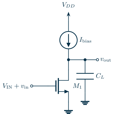
Let us size the common-source amplifier of Figure 6.6 in both processes. An ideal current source sets the bias current; in a real circuit it would be a PMOS current mirror (Chapter 8). The specification is:
- unity-gain frequency \(f_u\) = 50 MHz into \(C_L\) = 2 pF;
- low-frequency gain \(\lvert A_v\rvert \geq 30\) (29.5 dB), set by the transistor alone, \(\lvert A_v\rvert = g_m/g_{ds}\), since the ideal load has infinite resistance;
- output biased at \(V_{DD}/2\), so 0.6 V in SG13G2 and 0.9 V in SKY130;
- \(g_m/I_D = 15\ \mathrm{V^{-1}}\) (moderate inversion, a good starting point for an amplifying device).
Worked example 6.1 · Sizing the common-source stage
Step 1. \(g_m = 2\pi \cdot 50\ \mathrm{MHz} \cdot 2\ \mathrm{pF} = 628\ \mu\mathrm{S}\).
Steps 2 and 3. At \(g_m/I_D = 15\), \(I_D = 628\ \mu\mathrm{S}/15 = 41.9\ \mu\mathrm{A}\) in both PDKs.
Step 4. We need \(g_m/g_{ds} \geq 30\). In SG13G2 the gain chart gives 23.6 at 0.35 µm, 26.4 at 0.5 µm and 30.1 at 0.75 µm, so L = 0.75 µm. In SKY130 the minimum length gives only 22, but 0.18 µm already gives 42.9, so L = 0.18 µm. The transit frequencies are 1.10 GHz and 15.5 GHz, both well above 50 MHz.
Step 5. The width chart gives 2.32 µA/µm (SG13G2, L = 0.75 µm) and 9.07 µA/µm (SKY130, L = 0.18 µm), so W = 18.05 µm and W = 4.62 µm. SG13G2 fingers may be at most 10 µm wide, so the SG13G2 device becomes two fingers of 9.03 µm.
Step 6. The tables predict \(V_{GS}\) = 325 mV and 775 mV, input capacitances \(C_{gg}\) = 90.8 fF and 6.45 fF, and drain capacitances of 6.0 fF and 2.1 fF. Including the drain capacitance in the load, the predicted unity-gain frequencies are 49.9 MHz in both PDKs.
To simulate the stage we must hold its output at \(V_{DD}/2\). With an ideal current-source load the DC gain is around 30 to 40, so a 1 mV error in the gate voltage moves the output by 30 to 40 mV: no fixed gate voltage would put it at exactly mid-supply. The testbench therefore sets the gate bias with a very slow feedback loop, a DC servo, that adjusts \(V_{GS}\) until the output sits at \(V_{DD}/2\) and is open at every frequency of interest. Inside a real amplifier, the surrounding feedback does this job.
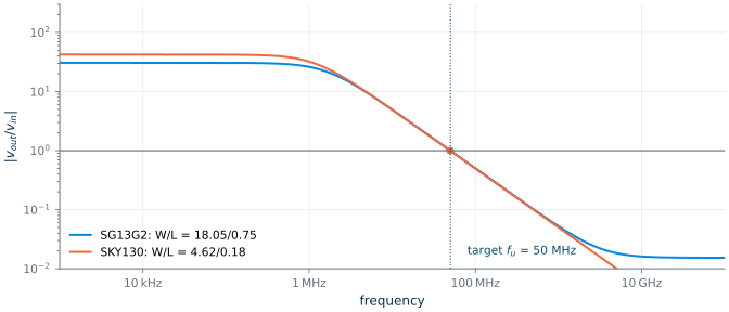
Table 6.1. Predicted and simulated performance of the common-source stage.
| Quantity | SG13G2 predicted | SG13G2 simulated | SKY130 predicted | SKY130 simulated |
|---|---|---|---|---|
| W/L (µm) | 18.05/0.75 (2 fingers) | 4.62/0.18 | ||
| \(V_{GS}\) | 325 mV | 311 mV | 775 mV | 775 mV |
| \(g_m\) | 628 µS | 633 µS | 628 µS | 622 µS |
| Gain \(g_m/g_{ds}\) | 30.1 | 30.7 | 42.9 | 42.4 |
| \(f_u\) | 49.9 MHz | 50.0 MHz | 49.9 MHz | 49.4 MHz |
The tables predicted gain and bandwidth to within 2 % in both processes, without a single fitted parameter. Figure 6.7 shows the simulated frequency responses. At very high frequencies the SG13G2 response flattens out at about 0.015. Here the input couples capacitively from gate to drain, past the transistor’s gain, and divides against the load. For this large device the coupling is about 31 fF: 8.8 fF of overlap capacitance plus 22 fF from the channel charge, which also responds to the gate voltage. We return to this feedforward path in Chapter 9.
What this means for your design
The two transistors meet the same specification with the same current, but they are very different devices. To reach a gain of 30, the SG13G2 transistor needs a 4× longer channel and is therefore 4× wider, so its gate capacitance is 14 times larger (90.8 fF against 6.45 fF). Whatever drives this stage in SG13G2 will see that capacitance as its load. The gm/ID method makes such consequences visible at step 6, before you draw a single schematic.
Common pitfall · Assuming every width scales like the table
The method rests on the claim that \(g_m/I_D\) depends on \(I_D/W\) and not on \(W\). That holds for wide devices, but transistor models also describe narrow-width effects, and the SKY130 models do it with separately fitted bins in W and L. At L = 0.18 µm and a fixed \(V_{GS}\), a 1 µm wide SKY130 NMOS carries 7.7 µA/µm, a 2 µm one 13.9 µA/µm and a 5 µm one 9.0 µA/µm, and the intrinsic gain jumps from 27 to 43 between 3 and 5 µm. Our first version of this example used \(C_L\) = 1 pF, which gave a 2.31 µm wide SKY130 device and a simulated gain of 26 instead of the predicted 43. In SG13G2 the change with width is smooth, but still about 20 % in current density between 2.3 and 5 µm. The cure is simple: keep each finger as wide as the device in the table, and reach larger widths with more fingers (
ngin SG13G2,nfin SKY130) or the multiplierm. If your design needs narrow fingers, build a table at that finger width.
6.7 Choosing the channel length
Of the three choices in Eq. (6.4), \(g_m\) comes from the specification and \(g_m/I_D\) from the device’s role. The length is where judgement comes in. Figure 6.8 summarizes the trade-off at \(g_m/I_D = 15\ \mathrm{V^{-1}}\).
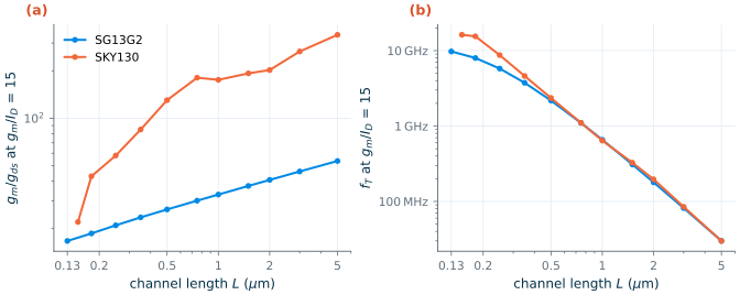
- Speed falls quickly with length. Above about 0.5 µm the transit frequency falls almost as \(1/L^2\) in both PDKs: from about 2.2 GHz at 0.5 µm to 30 MHz at 5 µm. The two processes are almost identical here, because at long lengths the speed is set by mobility and length, not by the fine detail of the process.
- Gain rises slowly with length, and how slowly depends on the process. SG13G2 goes from 17 at minimum length to 54 at 5 µm; SKY130 jumps from 22 to 130 by 0.5 µm and then climbs gently to 340.
- Area rises with length squared: at fixed \(I_D\) and \(g_m/I_D\), doubling L doubles W as well.
These lead to some practical starting points, which the later chapters refine:
| Device role | Starting L | Why |
|---|---|---|
| Signal-path amplifying devices | shortest L that meets the gain; often 2–4 × Lmin | speed and small capacitance |
| Current mirrors, tail and load current sources | 1–5 µm | high output resistance and good matching |
| Switches and digital gates | Lmin | low on-resistance and charge |
| SG13G2 devices that need gain | as long as speed allows, or cascode | intrinsic gain is limited to about 30–50 |
- The square law is accurate only above about 150 mV of overdrive, while most analog transistors today are biased in moderate inversion, below that. Design from simulated data instead.
- \(g_m/I_D\) measures the inversion level: about 30 V⁻¹ in weak inversion, falling to 3–5 V⁻¹ in strong inversion. It depends on current density, not width, so one table describes every width.
- Four charts (bias, width, speed, gain) contain everything needed to size a transistor; a lookup table holds them for every L and \(V_{DS}\).
- The recipe: \(g_m\) from the specification, \(g_m/I_D\) from the role, L from gain and speed, then \(I_D\), W, \(V_{GS}\) and the capacitances follow. In the worked example it predicted gain and bandwidth to within 2 %.
- SG13G2’s 1.2 V core devices have 3–5× less intrinsic gain than SKY130’s 1.8 V devices, so expect longer channels or cascodes in SG13G2.
- Keep finger widths equal to the table’s width, especially in SKY130, whose binned models break the width scaling at short lengths.
Further reading
- P. G. A. Jespers and B. Murmann, Systematic Design of Analog CMOS Circuits [56]: the complete treatment of lookup-table design, with many worked circuits.
- F. Silveira, D. Flandre and P. G. A. Jespers [74]: the short paper that started it all.
- B. Murmann’s starter kit [46] and pygmid [45]: ready-made tables and tools for SKY130 and SG13G2.
- H. Pretl et al., JKU analog circuit design course [2]: gm/ID design of complete circuits in SG13G2, with Jupyter notebooks.
- S. Palermo, ECEN 474, lecture on table-based design [1]: a compact lecture-sized introduction.
- C. C. Enz and E. A. Vittoz [59]: the EKV model and the inversion coefficient in depth.