Chapter 12
The Two-Stage Miller OTA
The course project: a two-stage Miller-compensated OTA designed to the same specification in SG13G2 and SKY130, sized with gm/ID, and verified for gain, bandwidth, stability, slew rate, range and rejection across process corners and temperature.
- Turn an amplifier specification into gain, bandwidth, slew-rate and swing budgets.
- Choose the input-pair polarity and the channel lengths from the supply and the process.
- Follow a step-by-step gm/ID procedure to size every transistor of a two-stage OTA, and check the hand predictions against the simulated operating point.
- Verify the design in both PDKs: loop gain, step response, output swing, input range, PSRR, CMRR and power.
- Run corners and temperature, and judge the design against its specification.
Contents
12.1 The specification
Every amplifier design starts from a table of numbers. Ours is the specification of the course project, the same in both processes. It applies at the nominal core supply (\(V_{DD}\) = 1.2 V in SG13G2, 1.8 V in SKY130), in the typical corner (tt) at 27 °C, unless a line says otherwise.
Table 12.1. Specification of the course OTA, and the test condition used to check each line.
| Specification | Target | How we check it |
|---|---|---|
| Load capacitance \(C_L\) | 2 pF | at the output in every testbench |
| Unity-gain bandwidth (GBW) | ≥ 20 MHz | unity-gain frequency \(f_u\) of the loop gain, follower connection |
| Phase margin (PM) | ≥ 60° (tt), ≥ 45° over corners | phase of the loop gain at \(f_u\) |
| DC open-loop gain \(A_0\) | ≥ 60 dB | loop gain at low frequency |
| Slew rate (SR) | ≥ 10 V/µs | 0.3 V step on the unity-gain follower |
| Output swing | 0.2 V to \(V_{DD}\) − 0.2 V | open-loop gain ≥ 54 dB (half the gain target) over this range |
| Bias | from a 10 µA reference current | ideal current source into the ibias port |
| Power | as low as possible | supply current × \(V_{DD}\) |
Three conventions make the numbers comparable between the PDKs. The input common-mode level is \(V_{CM} = V_{DD}/2\) (0.6 V and 0.9 V). The OTA is tested as a unity-gain follower, the most demanding configuration for stability, because the whole output is fed back (\(\beta\) = 1). And all loop gains are measured with the double-injection probe of Section 11.4, so the load the amplifier sees is always the real one.
Why two stages? Chapter 10 designed a five-transistor OTA for the same load and bandwidth. Its gain is roughly half the intrinsic gain \(g_m/g_{ds}\) of its transistors, which at the lengths that keep it fast is roughly 20–25 dB in SG13G2 and 35–40 dB in SKY130 (half the intrinsic gains of Section 6.3). Sixty decibels needs a second gain stage, and a second stage needs compensation. That is the subject of this chapter.
12.2 Architecture
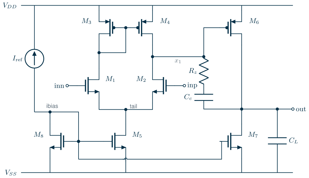
Figure 12.1 shows the circuit. The first stage is a differential pair \(M_{1,2}\) with a current-mirror load \(M_{3,4}\) and a tail source \(M_5\): the 5T OTA. Its output \(x_1\) drives the second stage, a common-source amplifier \(M_6\) with a current-source load \(M_7\). The Miller capacitor \(C_c\) in series with the nulling resistor \(R_z\) connects the output back to \(x_1\) (Sections 11.6 and 11.7). The 10 µA reference current enters the diode-connected \(M_8\), and \(M_5\) and \(M_7\) copy it with ratios of 2 and 6. Both stages invert, so inp is the non-inverting input.
Which input pair?
The first decision is the polarity of the input pair, and at these supplies it is decided by the input common-mode range (ICMR). An NMOS pair needs its tail transistor in saturation, so the input cannot go lower than \(V_{GS1} + V_{DS,sat5}\). A PMOS pair is the mirror image: the input cannot go higher than \(V_{DD} - \lvert V_{GS1}\rvert - \lvert V_{DS,sat5}\rvert\). Reading the gate voltages from the gm/ID tables of Chapter 6 at a moderate-inversion bias (\(g_m/I_D \approx 15\ \mathrm{V^{-1}}\)) and allowing about 0.2 V for the tail gives:
Table 12.2. Estimated input range of each pair polarity, from the gm/ID tables (no body effect).
| Quantity | SG13G2 (1.2 V) | SKY130 (1.8 V) |
|---|---|---|
| NMOS pair, \(V_{GS}\) at 15 V⁻¹ | 0.28–0.32 V | 0.67 V |
| NMOS pair: lowest input | ≈ 0.5 V | ≈ 0.85 V |
| PMOS pair, \(\lvert V_{GS}\rvert\) at 15 V⁻¹ | 0.43–0.45 V | 1.02–1.06 V |
| PMOS pair: highest input | ≈ 0.56 V | ≈ 0.55 V |
| \(V_{DD}/2\) | 0.6 V | 0.9 V |
In SKY130 the answer is clear. The 1.8 V PMOS has a threshold near 1 V, so a PMOS pair stops working at about 0.55 V, far below mid-supply. Only an NMOS pair can accept 0.9 V. In SG13G2 both polarities are tight: at 1.2 V each pair has an input range only about half a volt wide, and \(V_{DD}/2\) sits near the boundary between them. The NMOS pair keeps about 0.1 V of margin at 0.6 V, the PMOS pair has none. A second argument settles it. The SG13G2 PMOS has four to five times the intrinsic gain of the NMOS at the same length and \(g_m/I_D\) (Section 6.3 tables), and the NMOS-input topology puts PMOS transistors exactly where their output conductance limits the gain: the mirror load \(M_4\) and the second-stage driver \(M_6\). Both designs therefore use an NMOS input pair and a PMOS second stage. A PMOS input would be the better choice for a low common-mode level, or for low flicker noise (Chapter 13).
12.3 Design equations
The small-signal analysis of the two-stage OTA was done in Chapter 11. Here we collect the results we need for sizing, following the classic treatments [54, 51, 53]. Write \(R_1 = 1/(g_{ds2}+g_{ds4})\) and \(R_2 = 1/(g_{ds6}+g_{ds7})\) for the resistances at the two high-impedance nodes, and \(C_1\), \(C_2\) for their capacitances (\(C_2 \approx C_L\)).
Key equations · The two-stage Miller OTA
\[A_0 = g_{m2}R_1\cdot g_{m6}R_2 = \frac{(g_m/I_D)_2}{\lambda_2+\lambda_4}\cdot\frac{(g_m/I_D)_6}{\lambda_6+\lambda_7}, \qquad \lambda_k = \frac{g_{ds,k}}{I_{D,k}} = \frac{(g_m/I_D)_k}{(g_m/g_{ds})_k} \tag{12.1}\] \[\mathrm{GBW} = \frac{g_{m2}}{2\pi C_c} \tag{12.2}\] \[f_{p2} = \frac{g_{m6}\,C_c}{2\pi\left[C_1C_2 + C_c(C_1+C_2)\right]} \approx \frac{g_{m6}}{2\pi C_2}\ \ (C_c \gg C_1) \tag{12.3}\] \[f_{z} = \frac{1}{2\pi C_c\,(1/g_{m6}-R_z)} \tag{12.4}\] \[\mathrm{SR} \approx \min\!\left(\frac{I_{5}}{C_c},\ \frac{I_{7}}{C_c+C_L}\right) \tag{12.5}\] \[\mathrm{PM} \approx 90^\circ - \arctan\frac{f_u}{f_{p2}} - \arctan\frac{f_u}{f_{z}} - \sum\arctan\frac{f_u}{f_{p,k}} \tag{12.6}\]
Eq. (12.1) is the gm/ID form of the gain: each stage gives its transconductance efficiency divided by the sum of the “inverse Early voltages” \(\lambda\) of the two transistors at its output. Eq. (12.4) is the zero of the compensation branch: in the right half-plane for \(R_z < 1/g_{m6}\), at infinity for \(R_z = 1/g_{m6}\), and in the left half-plane above that, where it adds phase instead of removing it. In Eq. (12.6) the sum runs over the remaining poles, mainly the mirror pole at node \(d_1\), \(f_{p3} \approx g_{m3}/(2\pi\cdot 2C_{gg3})\). A sign convention: \(f_z\) is negative (left half-plane) when \(R_z > 1/g_{m6}\), which turns its arctangent into a phase lead.
Two large-signal conditions complete the set. The output can swing from \(V_{DS,sat7}\) to \(V_{DD}-\lvert V_{DS,sat6}\rvert\), and the input common-mode range is
\[V_{GS1} + V_{DS,sat5} \;\le\; V_{CM} \;\le\; V_{DD} - \lvert V_{GS3}\rvert + V_{TH1}. \tag{12.7}\]Finally, the output must sit near mid-supply when the inputs are equal, otherwise the amplifier has a systematic offset. With the inputs equal, \(x_1\) sits at the drain voltage of the diode \(M_3\), so \(M_6\) has the same \(V_{GS}\) as \(M_4\). If they also have the same length, their currents scale with width, and the current of \(M_6\) must equal the one \(M_7\) is forced to carry:
\[\frac{W_6}{W_4} = \frac{I_7}{I_5/2} = 2\,\frac{W_7}{W_5}. \tag{12.8}\]The demo below puts these equations to work on the course OTA of Sections 12.5 and 12.6. Move \(C_c\) and \(R_z\), or pick a preset, and watch the loop gain, the phase margin and the step response of the OTA connected as a follower.
12.4 A gm/ID design procedure
The procedure has seven steps. Steps 1–3 set currents and transconductances from bandwidth and slew rate; step 4 sets the lengths from gain; steps 5–7 turn everything into widths and check it. It follows the gm/ID recipe of Section 6.5 and the two-stage procedures of Jespers and Murmann [56] and Allen and Holberg [54]. The code is in tools/figs/_ch12_ota.py (function design).
- Choose \(C_c\) and the GBW target. A rule of thumb from pole splitting is \(C_c \approx 0.2\)–\(0.5\,C_L\): smaller, and \(f_{p2}\) in Eq. (12.3) collapses once \(C_c\) approaches \(C_1\); larger, and the input pair needs more current for the same GBW. We take \(C_c = C_L/2 = 1\) pF, and design for a GBW of 25 MHz, 25 % above the specification, because \(f_u\) comes out below \(g_{m2}/(2\pi C_c)\) when \(f_{p2}\) is only about twice as high.
- Input pair and tail. Eq. (12.2) gives \(g_{m2}\) = 157 µS. The slew rate needs \(I_5 \ge \mathrm{SR}\cdot C_c\) = 10 µA. We take \(I_5\) = 20 µA, twice the reference, so each side carries 10 µA and the pair runs at \(g_m/I_D\) = 15.7 V⁻¹: moderate inversion, a good compromise between efficiency, noise and the size of the pair.
- Second stage. For a phase margin above 60° we place \(f_{p2}\) at about twice the GBW and let the left-half-plane zero of \(R_z\) provide the rest. With \(C_1 \approx 0.3\) pF, Eq. (12.3) asks for \(g_{m6} \approx\) 0.9–1 mS. The output slew rate needs \(I_7 \ge \mathrm{SR}(C_L+C_c)\) = 30 µA. We take \(I_7\) = 60 µA (six times the reference), which gives 20 V/µs and puts \(M_6\) at \(g_m/I_D \approx\) 13–16 V⁻¹. The swing limit of 0.2 V sets the saturation voltages of \(M_6\) and \(M_7\) below about 0.18 V, so neither can sit deep in strong inversion: \(g_m/I_D \ge 11\ \mathrm{V^{-1}}\).
- Lengths from the gain. Eq. (12.1) tells us which transistors matter: \(M_2\) and \(M_4\) in the first stage, \(M_6\) and \(M_7\) in the second. Lengthen the ones whose \(\lambda\) dominates, as long as their capacitance does not hurt the speed. This step is where the two processes part ways (Sections 12.5 and 12.6).
- Widths. Read the current density at each \(g_m/I_D\), L and \(V_{DS}\) from the tables and divide. Split the result into fingers: in SG13G2 we keep fingers at or below 5 µm with even counts in the matched groups; in SKY130 every finger is exactly 5 µm, the width of the table, because of the model’s width bins (Section 6.6). Within each mirror (\(M_{3,4,6}\) and \(M_{5,7,8}\)) the finger width is the same, so the ratios of Eq. (12.8) are exact finger counts.
- Nulling resistor. Eq. (12.4) gives \(1/g_{m6}\) (zero at infinity) and \((1+C_2/C_c)/g_{m6}\) (zero on top of \(f_{p2}\)). We start halfway between them, which places a left-half-plane zero at a few times \(f_u\) and leaves room for corners; Figure 11.8 shows how the phase margin depends on this choice.
- Check the operating point in simulation against the predictions (Table 12.4), then verify the whole specification (Section 12.7).
Worked example 12.1 · The SG13G2 budget by hand
Steps 1–2. \(g_{m2} = 2\pi\cdot 25\ \mathrm{MHz}\cdot 1\ \mathrm{pF} = 157\ \mu\mathrm{S}\); with 10 µA per side, \(g_m/I_D = 15.7\ \mathrm{V^{-1}}\). Slew rate from the tail: \(20\ \mu\mathrm{A}/1\ \mathrm{pF} = 20\) V/µs.
Step 3. \(M_6\) at \(g_m/I_D = 16\ \mathrm{V^{-1}}\) and 60 µA gives \(g_{m6}\) = 960 µS. Its gate capacitance (L = 0.5 µm, \(f_T\) = 507 MHz) is \(C_{gg6} = g_{m6}/(2\pi f_T)\) = 301 fF; with the drains of \(M_2\) and \(M_4\), \(C_1\) = 311 fF. Eq. (12.3): \(f_{p2} = \dfrac{0.96\ \mathrm{mS}\cdot 1\ \mathrm{pF}}{2\pi\,[0.311\cdot 2.0 + 1\cdot(0.311+2.0)]\ \mathrm{pF^2}}\) = 51 MHz, about twice the GBW.
Step 4. At the expected drain voltages the tables give intrinsic gains of 39 for \(M_2\) (NMOS, L = 3 µm), 91 for \(M_4\) and 126 for \(M_6\) (PMOS, L = 0.5 µm), and 53 for \(M_7\) (NMOS, L = 5 µm, 11 V⁻¹). Eq. (12.1): \(\lambda_2\) = 15.7/39 = 0.40, \(\lambda_4\) = 0.18, \(\lambda_6\) = 0.13, \(\lambda_7\) = 0.21 V⁻¹, so \(A_1 = 15.7/0.58 = 27.3\) and \(A_2 = 16/0.34 = 47.7\): \(A_0\) = 1300 = 62.3 dB.
Step 6. \(1/g_{m6}\) = 1.04 kΩ and \((1 + C_2/C_c)/g_{m6}\) = 3.2 kΩ; halfway, \(R_z\) = 2.1 kΩ.
Simulation. The loop gain of Section 12.7 gives \(A_0\) = 62.2 dB, \(f_u\) = 21.5 MHz and PM = 67°. The gain prediction is within 0.1 dB. The unity-gain frequency is 14 % below \(g_{m2}/(2\pi C_c)\), as step 1 anticipated: the second pole and the mirror pole bend the gain curve down just before it crosses unity.
12.5 The SG13G2 design
In SG13G2 the gain is the hard part. The intrinsic gain of the 1.2 V NMOS is only 20–50 even at long channels (Section 6.3), and an NMOS sits in the gain path of each stage: \(M_2\) in the first, \(M_7\) in the second. Three measures together bring the gain above 60 dB.
- Long NMOS current sources. \(M_5\), \(M_7\) and \(M_8\) use L = 5 µm. They carry DC only, so their large gate capacitance (2.4 pF for \(M_7\)) hangs on the quiet bias node, not in the signal path. \(M_7\) runs at \(g_m/I_D = 11\ \mathrm{V^{-1}}\), the lowest value the swing allows, because \(\lambda = (g_m/I_D)/(g_m/g_{ds})\) falls with \(g_m/I_D\) while the NMOS intrinsic gain hardly changes.
- PMOS devices in weak-to-moderate inversion. \(M_{3,4,6}\) run at 16 V⁻¹ with L = 0.5 µm. A lower \(\lvert V_{GS3}\rvert\) lifts node \(x_1\), which gives \(M_2\) a larger \(V_{DS}\) and therefore a smaller \(g_{ds2}\).
- A long input pair. The pair length is the remaining knob, and Figure 12.2 shows what it costs.
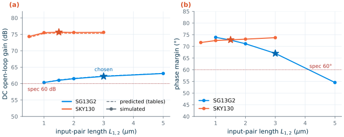
Lengthening the pair from 1 to 5 µm raises the gain by only 2.8 dB (60.3 to 63.1 dB), because the NMOS intrinsic gain grows slowly with length. The price grows quickly. At constant \(g_m/I_D\) the width grows with L, so the gate capacitance of each pair transistor rises from 41 fF at 1 µm to 330 fF at 3 µm and 900 fF at 5 µm. In the follower that capacitance loads the output and sits between the input and \(x_1\), and the phase margin falls from 74° to 55°. We choose L = 3 µm: 62.2 dB at tt, and, as Section 12.8 shows, at least 60.9 dB at every corner, against 59 dB at 125 °C for the 1 µm pair.
SG13G2 vs SKY130 · Where the gain comes from
In SG13G2 the first stage gives a gain of 27 and the second 48. In SKY130 both stages give about 75, with shorter devices. The 2.2 dB of SG13G2 margin above 60 dB at tt (0.9 dB at the worst corner) is all there is: a cascode would add 20–30 dB, but a cascoded NMOS sink at the output needs about 0.3 V of headroom, which breaks the 0.2 V swing specification at 1.2 V, and a cascoded first stage needs another bias voltage and narrows the input range further. These are the standard next steps if your SG13G2 application needs more gain: a folded or telescopic cascode first stage, or a gain-boosted cascode [51, 62]. The 3.3 V thick-oxide devices of SG13G2 are not an option inside a 1.2 V amplifier.
12.6 The SKY130 design
SKY130 has gain to spare: Eq. (12.1) predicts 75 dB with a 1.5 µm pair, 0.5 µm PMOS devices and 2 µm current sources. The design is shaped instead by the model’s width bins: every device is built from 5 µm fingers, so step 5 fixes the widths and the gm/ID values follow from the resulting current density. With 2 fingers per pair transistor (10 µm, 1 µA/µm), the pair lands at 15.6 V⁻¹ and \(g_{m2}\) = 156 µS, which is the 25 MHz target. Figure 12.2 shows that in SKY130 the pair length hardly changes the gain (74.3 dB at 0.5 µm, 75.7 dB at 1.5 µm); with the width fixed at 10 µm it mainly sets \(g_m/I_D\), and 1.5 µm lands on the GBW target with \(C_c\) = 1 pF.
Common pitfall · Simulating SKY130 without the reference .spiceinit
Binned models such as SKY130’s contain several parameter sets, each fitted for a range of W and L, and the simulator picks one per device. For a multi-finger device the choice must use the finger width W/nf. ngspice does this only in its HSPICE-compatibility mode, which IIC-OSIC-TOOLS switches on in its
~/.spiceinit(set ngbehavior=hsa, together withset ng_nomodcheckandset enable_noisy_r); without it, BSIM4 selects the bin from the total width. Our first SKY130 runs used a bare local ngspice and showed exactly this. For an NMOS at L = 1 µm, 1 µA/µm and \(V_{DS}\) = 0.53 V, one 5 µm finger gave \(g_m/g_{ds}\) = 146, but two 5 µm fingers (W = 10 µm, nf = 2) gave 51; at L = 2 µm, four fingers gave 150 instead of 168. Withngbehavior=hsa, every finger count agrees with the single finger. The OTA with a 1 µm pair simulated 69.4 dB instead of the 75.3 dB the tables predicted; with the setting it gives 75.5 dB. The tables, built from one finger, were right; the simulator setup was wrong. Two lessons: run ngspice with the same.spiceinitas the PDK’s reference environment (ourtools/aicd/spice.pynow writes it for local runs), and always compare the simulated operating point with the table predictions, device by device (Table 12.4). A disagreement by a factor of three points to the setup, not to the design.
The complete sizes of both designs are in Table 12.3, and the operating points in Table 12.4.
Table 12.3. Device sizes. W is the total width, split into the given number of fingers. Currents are design values.
| Device | Role | \(I_D\) | SG13G2 W/L (µm), fingers | SKY130 W/L (µm), fingers |
|---|---|---|---|---|
| \(M_{1,2}\) | input pair | 10 µA | 18.2/3, 4 × 4.55 | 10/1.5, 2 × 5 |
| \(M_{3,4}\) | mirror load | 10 µA | 13.32/0.5, 4 × 3.33 | 10/0.5, 2 × 5 |
| \(M_5\) | tail | 20 µA | 22.56/5, 8 × 2.82 | 20/2, 4 × 5 |
| \(M_6\) | second stage | 60 µA | 79.92/0.5, 24 × 3.33 | 60/0.5, 12 × 5 |
| \(M_7\) | output sink | 60 µA | 67.68/5, 24 × 2.82 | 60/2, 12 × 5 |
| \(M_8\) | bias diode | 10 µA | 11.28/5, 4 × 2.82 | 10/2, 2 × 5 |
| \(C_c\), \(R_z\) | compensation | 1 pF, 2.1 kΩ | 1 pF, 2.6 kΩ |
Table 12.4. Operating point at tt, 27 °C: hand prediction from the tables / simulation.
| Quantity | SG13G2 | SKY130 |
|---|---|---|
| \(I_{D2}\) (µA) | 10.0 / 9.8 | 10.0 / 9.4 |
| \(g_m/I_D\) of \(M_2\) (V⁻¹) | 15.7 / 15.8 | 15.6 / 16.0 |
| \(g_m/g_{ds}\) of \(M_2\), \(M_4\) | 39 / 38, 91 / 94 | 154 / 162, 135 / 137 |
| \(I_{D6}\) (µA) | 60 / 63.5 | 60 / 61.1 |
| \(g_{m6}\) (µS) | 960 / 1010 | 783 / 793 |
| \(g_m/g_{ds}\) of \(M_6\), \(M_7\) | 126 / 126, 53 / 53 | 127 / 126, 202 / 202 |
| \(C_{gg}\) of \(M_2\), \(M_6\) (fF) | 330 / 321, 301 / 293 | 83 / 82, 154 / 155 |
| \(A_0\) (dB) | 62.3 / 62.2 | 75.4 / 75.7 |
| Output offset (systematic) | — / −0.1 mV | — / −0.1 mV |
The agreement is within a few percent everywhere. The 6 % excess current in the SG13G2 \(M_6\) comes from Eq. (12.8)’s hidden assumption that \(M_4\) and \(M_6\) see the same \(V_{DS}\): \(M_4\) sits at 0.44 V and \(M_6\) at 0.6 V, and the low output resistance of SG13G2 devices turns that difference into current. In the follower the loop absorbs it, at the price of a systematic offset of only 0.1 mV.
The subcircuits are saved as tools/figs/ch12_ota_sg13g2.spice and tools/figs/ch12_ota_sky130.spice; Chapters 13, 15 and 16 and Labs 6–8 start from them. The core of each:
* two-stage Miller OTA, SG13G2 (needs .lib cornerMOSlv.lib mos_tt)
.subckt ota2s inp inn out vdd vss ibias
XM1 d1 inn tail vss sg13_lv_nmos W=18.2u L=3u ng=4 m=1
XM2 x1 inp tail vss sg13_lv_nmos W=18.2u L=3u ng=4 m=1
XM3 d1 d1 vdd vdd sg13_lv_pmos W=13.32u L=0.5u ng=4 m=1
XM4 x1 d1 vdd vdd sg13_lv_pmos W=13.32u L=0.5u ng=4 m=1
XM5 tail ibias vss vss sg13_lv_nmos W=22.56u L=5u ng=8 m=1
XM6 out x1 vdd vdd sg13_lv_pmos W=79.92u L=0.5u ng=24 m=1
XM7 out ibias vss vss sg13_lv_nmos W=67.68u L=5u ng=24 m=1
XM8 ibias ibias vss vss sg13_lv_nmos W=11.28u L=5u ng=4 m=1
Rz x1 xz 2100
Cc xz out 1e-12
.ends ota2s
* two-stage Miller OTA, SKY130 (needs .lib .../sky130.lib.spice tt; W, L in um)
* diffusion areas (ad, as, pd, ps) as written by tools/aicd/pdk.py are omitted here for brevity
.subckt ota2s inp inn out vdd vss ibias
XM1 d1 inn tail vss sky130_fd_pr__nfet_01v8 W=10 L=1.5 nf=2
XM2 x1 inp tail vss sky130_fd_pr__nfet_01v8 W=10 L=1.5 nf=2
XM3 d1 d1 vdd vdd sky130_fd_pr__pfet_01v8 W=10 L=0.5 nf=2
XM4 x1 d1 vdd vdd sky130_fd_pr__pfet_01v8 W=10 L=0.5 nf=2
XM5 tail ibias vss vss sky130_fd_pr__nfet_01v8 W=20 L=2 nf=4
XM6 out x1 vdd vdd sky130_fd_pr__pfet_01v8 W=60 L=0.5 nf=12
XM7 out ibias vss vss sky130_fd_pr__nfet_01v8 W=60 L=2 nf=12
XM8 ibias ibias vss vss sky130_fd_pr__nfet_01v8 W=10 L=2 nf=2
Rz x1 xz 2600
Cc xz out 1e-12
.ends ota2s
12.7 Verification
Verification means checking every line of Table 12.1 with a testbench that a reviewer could rerun. The stand-alone testbenches ch12_tb_sg13g2.spice and ch12_tb_sky130.spice run in IIC-OSIC-TOOLS with ngspice -b and print \(A_0\), \(f_u\), the phase margin and the rising slew rate; they use the loop-gain probe of Section 11.4. The figures below come from the Python version of the same benches in tools/figs/ch12_two_stage.py.
Loop gain: DC gain, bandwidth and phase margin
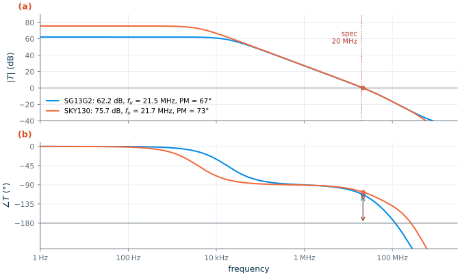
Figure 12.3 shows the loop gain of the follower. Both amplifiers cross unity just above the 20 MHz line, at 21.5 MHz (SG13G2) and 21.7 MHz (SKY130), with phase margins of 67° and 73° and gain margins of 18.5 dB and 28.4 dB. The dominant pole sits at 19 kHz in SG13G2 and 4 kHz in SKY130: the higher gain of SKY130 pushes it lower, so that the gain-bandwidth product stays the same. That is Eq. (12.2) at work: GBW depends on \(g_{m2}\) and \(C_c\) only.
Large-signal step: slew rate and settling
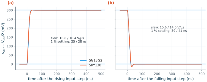
Figure 12.4 shows the follower’s response to a 0.3 V step up from \(V_{DD}/2\) and back. On the rising edge the output slews at 16.8 V/µs (SG13G2) and 16.4 V/µs (SKY130), close to the internal limit \(I_5/C_c\) = 20 V/µs of Eq. (12.5); on the falling edge, where \(M_7\) must discharge \(C_L + C_c\) with its fixed 60 µA, at 15.6 and 14.6 V/µs (the limit is 20 V/µs). The measured values are the slopes between 20 % and 80 % of the step, which include the start of linear settling and so read a little lower than the pure slewing rate. The output settles to 1 % in 25–28 ns after a rising step and 39–41 ns after a falling one, with a 5 % undershoot on the falling edge, where the amplifier comes out of slewing.
Output swing and input range
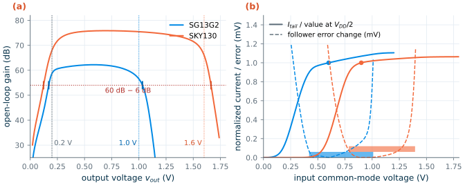
The output swing is measured open loop: with inn at \(V_{CM}\), a DC sweep of a few millivolts on inp drives the output from rail to rail, and the derivative of the transfer curve is the gain at every output voltage (Figure 12.5a). The gain stays above 54 dB, half the 60 dB target, from 0.17 to 1.03 V in SG13G2 and from 0.12 to 1.66 V in SKY130, so both meet the swing specification. At the specified limits of 0.2 V and \(V_{DD}\) − 0.2 V the gain is 58.7 and 56.5 dB in SG13G2 and 68.0 and 66.0 dB in SKY130. The gain falls where \(M_7\) (bottom) or \(M_6\) (top) leaves saturation, as Eq. (12.7)’s output-range estimate predicts.
The input range is measured in the follower by sweeping the input from 0 to \(V_{DD}\) (Figure 12.5b). At the bottom the tail transistor leaves saturation and its current falls; we take the point where it has fallen by 10 %. At the top \(M_2\) leaves saturation, the gain collapses and the follower stops following; we take the point where its error has grown by 1 mV. The input range is 0.42 to 1.01 V in SG13G2 and 0.79 to 1.40 V in SKY130. Mid-supply lies inside both, with 180 mV and 115 mV of margin at the bottom, as Table 12.2 anticipated.
Rejection and power
Two more AC analyses on the follower give the supply and common-mode rejection. For PSRR, a 1 V AC source in series with the supply appears at the output attenuated by the PSRR, because the closed-loop gain is one. For CMRR, the same AC source in series with both inputs gives \(v_{out}/v_c \approx A_{cm}/A_{dm} = 1/\mathrm{CMRR}\). Table 12.5 collects the results at tt and 27 °C. PSRR from the positive supply drops to 27 dB at 1 MHz in both PDKs: above the dominant pole \(C_c\) ties the gate of \(M_6\) to the output, so \(M_6\) acts as a diode from \(V_{DD}\) to the output and supply ripple passes through, a known weakness of this topology [53].
Table 12.5. Simulated performance at tt, 27 °C, against the specification.
| Quantity | Spec | SG13G2 | SKY130 |
|---|---|---|---|
| DC gain \(A_0\) | ≥ 60 dB | 62.2 dB ✓ | 75.7 dB ✓ |
| Unity-gain frequency \(f_u\) | ≥ 20 MHz | 21.5 MHz ✓ | 21.7 MHz ✓ |
| Phase margin | ≥ 60° | 67.0° ✓ | 72.8° ✓ |
| Gain margin | 18.5 dB | 28.4 dB | |
| Slew rate (rise / fall) | ≥ 10 V/µs | 16.8 / 15.6 V/µs ✓ | 16.4 / 14.6 V/µs ✓ |
| 1 % settling, 0.3 V step (rise / fall) | 25 / 39 ns | 28 / 41 ns | |
| Output swing (gain ≥ 54 dB) | 0.2 V to \(V_{DD}\) − 0.2 V | 0.17–1.03 V ✓ | 0.12–1.66 V ✓ |
| Input common-mode range | 0.42–1.01 V | 0.79–1.40 V | |
| PSRR+ / PSRR− at 1 kHz | 67.8 / 77.2 dB | 77.0 / 73.1 dB | |
| CMRR at 1 kHz | 65.8 dB | 72.0 dB | |
| Supply current, power | low | 93 µA, 112 µW | 90 µA, 162 µW |
The two designs draw almost the same current, 10 + 20 + 60 µA plus the small excess of \(M_6\), so the power simply scales with the supply. The SG13G2 design meets the specification at two thirds of the SKY130 power. That is the reward of the lower supply; the price is the thin gain margin of Section 12.5.
12.8 Corners and temperature
A design that works only at tt and 27 °C is not finished. We repeat the loop gain, the step and the operating point at the five process corners of each PDK (Chapter 3), tt, ss, ff, sf and fs, each at −40, 27 and 125 °C: 15 simulations per PDK. Figure 12.6 shows the results.
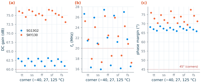
Table 12.6. Worst and best values over 5 corners × 3 temperatures, and the verdict.
| Quantity | Spec | SG13G2 range | SKY130 range | Verdict |
|---|---|---|---|---|
| DC gain | ≥ 60 dB | 60.9–63.1 dB | 73.1–76.6 dB | pass (SG13G2 by 0.9 dB) |
| Phase margin | ≥ 45° | 65.9–68.6° | 69.4–77.7° | pass |
| \(f_u\) | ≥ 20 MHz (tt) | 15.9–27.4 MHz | 17.2–26.2 MHz | pass at 27 °C; 16–19 MHz at 125 °C |
| Slew rate (worse edge) | ≥ 10 V/µs | 14.4–16.4 V/µs | 13.6–15.3 V/µs | pass |
| Power | 110–113 µW | 160–163 µW |
Process corners barely matter. The bias currents come from an ideal 10 µA reference, so they are the same at every corner, and the gm/ID design makes the transconductances depend on current rather than on threshold voltage. Temperature matters more. At constant current, \(g_m/I_D\) falls as the thermal voltage \(kT/q\) rises, from 20 mV at −40 °C to 34 mV at 125 °C, and carrier mobility falls too. The unity-gain frequency, \(g_{m2}/(2\pi C_c)\), therefore drops by 17–25 % from 27 °C to 125 °C, to 16 MHz in SG13G2 and 18 MHz in SKY130. The phase margin hardly moves, because \(g_{m6}\) and with it \(f_{p2}\) fall in the same proportion.
What this means for your design
The specification asks for 20 MHz at 27 °C, so both designs pass. If your system needs 20 MHz at 125 °C, two remedies exist. The brute-force one is 30 % more GBW at room temperature (more current or a smaller \(C_c\)). The elegant one is a bias current that rises with temperature so that \(g_{m2}\) stays constant: a constant-gm bias, which makes \(g_m\) track a resistor instead of \(kT/q\) (Chapter 8 and Chapter 14). The reference you design in Chapter 14 replaces the ideal 10 µA source here.
12.9 Design review
A design review asks three questions: does it meet the specification, where is the margin thin, and what would we change next?
- Specification. Both designs meet every line of Table 12.1 at tt and 27 °C, and the gain and phase margin hold over all fifteen corner–temperature combinations.
- Thin margins. SG13G2’s gain is 0.9 dB above the limit at the worst corner, and its output swing has little room at the top. Both designs lose 17–25 % of their bandwidth at 125 °C with a temperature-independent bias. PSRR from \(V_{DD}\) is poor above 1 MHz, a property of the PMOS-driver, Miller-compensated topology.
- What is not yet included. Noise and offset from mismatch (Chapter 13), a real bias reference (Chapter 14), and the parasitics of the layout (Chapters 15 and 16). The ideal \(C_c\) and \(R_z\) become a metal-insulator-metal capacitor and a poly resistor; their own parasitics move \(f_z\), so the phase margin must be checked again after extraction.
The gm/ID method earned its keep: with three choices per transistor, the hand predictions of Table 12.4 landed within a few percent of simulation, and the one large disagreement we met on the way (Section 12.6) pointed straight at a simulator-setup problem rather than a design error. All the numbers of this chapter are saved in tools/figs/ch12_numbers.json.
Try it · Lab 6
Lab 6 rebuilds this OTA in Xschem for your PDK, runs the testbench of Section 12.7 and the corner sweep, and then asks you to redesign it for a 40 MHz GBW at the same phase margin. Before you simulate, use Eqs. (12.1)–(12.5) to predict how much current the change costs.
- A specification becomes a design through budgets: GBW and \(C_c\) set \(g_{m2}\), slew rate sets the currents, phase margin sets \(g_{m6}\), gain sets the lengths, swing limits \(g_m/I_D\) from below.
- At 1.2 and 1.8 V the input common-mode range decides the pair polarity: SKY130’s 1 V PMOS threshold rules out a PMOS pair at mid-supply, and in SG13G2 the NMOS pair keeps the margin and puts the high-gain PMOS devices where they help.
- Gain \(= \prod (g_m/I_D)/\sum\lambda\): lengthen the devices whose \(\lambda\) dominates. In SG13G2 that means long NMOS current sources and a 3 µm input pair, which costs phase margin and input capacitance; SKY130 reaches 75 dB with short devices.
- Compare every device’s simulated operating point with its table prediction; here they agree within a few percent. A large disagreement usually means a setup error: SKY130 multi-finger devices need ngspice’s
set ngbehavior=hsa(as in IIC-OSIC-TOOLS’s.spiceinit), or BSIM4 picks the model bin from the total width.- Both designs meet the specification at tt and hold gain and phase margin over corners; bandwidth falls by up to a quarter at 125 °C unless the bias tracks temperature.
Further reading
- P. E. Allen and D. R. Holberg, CMOS Analog Circuit Design [54]: the classic step-by-step two-stage op-amp design procedure, in square-law form.
- P. G. A. Jespers and B. Murmann, Systematic Design of Analog CMOS Circuits [56]: two-stage amplifier design with lookup tables, including the optimum choice of \(C_c\).
- B. Razavi, Design of Analog CMOS Integrated Circuits [51]: two-stage op amps, compensation and the alternatives (folded and telescopic cascodes).
- P. R. Gray, P. J. Hurst, S. H. Lewis and R. G. Meyer [53]: the most thorough analysis of the two-stage op amp, including PSRR and slew rate.
- H. Pretl et al., JKU analog circuit design course [2]: a gm/ID-designed OTA in SG13G2 with complete Xschem and ngspice files.