Chapter 21
Data Converters
A data converter turns a voltage into a number, or a number into a voltage. Its accuracy is limited first by quantization, which no circuit can avoid, then by the mismatch, noise and distortion of the circuits that do the converting. This chapter defines the measures of a converter's accuracy, surveys the main converter architectures, and designs a successive-approximation ADC in both PDKs from the switches, capacitors and comparator of Chapters 18 to 20.
- Compute the quantization noise of an ideal converter and its signal-to-quantization-noise ratio.
- Define offset, gain error, DNL and INL, and SNR, SNDR, SFDR and ENOB, and measure them.
- Explain how resistor-string, current-steering and charge-redistribution DACs work, and predict the linearity of a capacitor DAC from the matching of its unit capacitor.
- Compare flash, successive-approximation, pipelined and delta-sigma ADCs, and explain how oversampling and noise shaping trade speed for resolution.
- Design and simulate a charge-redistribution SAR ADC, and read its waveforms, spectrum and energy per conversion.
Contents
Further learning · Open-BioAFE: data converters for a biomedical chip
This chapter introduces the converters; BRICD’s Open-BioAFE Tutorial designs them for a real chip, an eight-channel biopotential front-end in IHP SG13G2. Its Part III, Data Converters, continues from here: sampling and quantization, specifications and figures of merit, sample-and-hold circuits and switches, comparators, capacitive DACs and references, the SAR ADC, ΔΣ theory and ΔΣ circuits, converters made for biosignals and how to test an ADC, towards a 12-bit SAR and a 16-bit incremental ΔΣ ADC for microvolt ECG, EEG and EMG signals.
21.1 What a data converter does
An analog-to-digital converter (ADC) takes samples of its input at a sampling frequency \(f_s\), compares each sample with a set of reference levels and outputs the number of the level it falls into, a code of \(N\) bits. A digital-to-analog converter (DAC) does the opposite: it turns each code into one of \(2^N\) voltages or currents. Both divide a full-scale range \(V_{FS}\) into \(2^N\) steps of one least significant bit,
\[\mathrm{LSB} = \frac{V_{FS}}{2^N}. \tag{21.1}\]The converter of Section 21.7 has 8 bits and a full scale equal to the supply: its LSB is 4.69 mV in SG13G2 and 7.03 mV in SKY130. The sampling theorem asks for \(f_s\) at least twice the highest frequency in the signal. A Nyquist-rate converter samples close to that limit and resolves every sample to \(N\) bits; an oversampling converter samples much faster and gains its resolution by averaging, as Section 21.6 shows. Chapter 19 covered the sampling; this chapter is about the rest.
21.2 Quantization noise
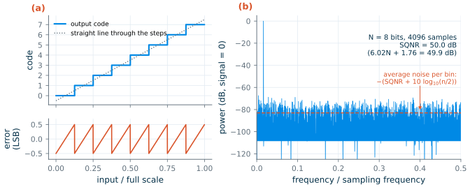
Even a perfect ADC makes an error: every input between two transition levels gives the same code. Figure 21.1a shows the transfer curve of an ideal 3-bit converter and its quantization error, a sawtooth between −½ and +½ LSB. If the input is busy enough that the error is equally likely anywhere in that range, the error behaves like a noise with a uniform distribution [108], whose power is
\[\overline{e_q^2} = \frac{\mathrm{LSB}^2}{12}. \tag{21.2}\]A full-scale sine has an amplitude of \(V_{FS}/2\) and a power of \(V_{FS}^2/8\). Dividing by Eq. (21.2):
Key equation · Signal-to-quantization-noise ratio
\[\mathrm{SQNR} = 10\log_{10}\frac{V_{FS}^2/8}{V_{FS}^2/(12\cdot 4^N)} = 6.02\,N + 1.76\ \mathrm{dB}. \tag{21.3}\]Each bit is worth 6 dB. An ideal 8-bit converter reaches 49.9 dB, a 12-bit one 74.0 dB, for a full-scale sine.
Figure 21.1b checks Eq. (21.3) with an ideal 8-bit quantizer and a coherently sampled sine: 50.0 dB. The quantization noise spreads over all the FFT bins from 0 to \(f_s/2\), so with \(n\) samples the floor of the spectrum lies \(10\log_{10}(n/2)\) below the total, 83 dB below the signal for 4096 samples. A small spur far below the signal says nothing about the SQNR unless the number of samples is known. The uniform-noise model fails for simple inputs, such as a DC level or a sine whose frequency is a simple fraction of \(f_s\): then the error repeats, and appears as harmonics instead of noise. Tests therefore use coherent sampling with \(f_{in} = (m/n)f_s\), where \(m\) and \(n\) have no common factor, so that every sample falls at a different phase of the sine.
21.3 Static accuracy: offset, gain, DNL and INL
A real converter’s transfer curve differs from the ideal one. Its offset shifts the whole curve, and its gain error changes its slope; both are usually removed by trimming or by a calibration in the digital domain, and do not limit the resolution. What remains is the nonlinearity of the steps [114]. For a DAC whose output for code \(k\) is \(V_k\) (for an ADC, \(V_k\) is the transition level into code \(k\)), with the average step \(\overline{\mathrm{LSB}} = (V_{2^N-1} - V_0)/(2^N - 1)\):
\[\mathrm{DNL}_k = \frac{V_{k+1} - V_k}{\overline{\mathrm{LSB}}} - 1, \tag{21.4}\] \[\mathrm{INL}_k = \frac{V_k - V_0}{\overline{\mathrm{LSB}}} - k. \tag{21.5}\]The differential nonlinearity (DNL) is the error of each step, in LSB; the integral nonlinearity (INL) is the distance of each level from the straight line through the end points, the sum of the DNL so far. These definitions remove offset and gain error by construction. A DNL of −1 LSB is a step of zero width, a missing code of an ADC; a DAC whose output falls when the code rises is non-monotonic. A converter whose \(\vert\mathrm{DNL}\vert\) stays below ½ LSB has neither. The INL is what distorts a large signal, since it bends the transfer curve.
21.4 Dynamic accuracy: SNDR, SFDR and ENOB
The dynamic measures come from the spectrum of the output for a sine input, as in Figure 21.1b. The signal-to-noise ratio (SNR) counts the noise in all bins except the signal and its harmonics; the total harmonic distortion (THD) counts the harmonics; the signal-to-noise-and-distortion ratio (SNDR or SINAD) counts everything that is not the signal; the spurious-free dynamic range (SFDR) is the ratio of the signal to the largest spur. The SNDR of a real converter is lower than Eq. (21.3), and the effective number of bits turns it back into the resolution of an ideal converter with the same SNDR:
\[\mathrm{ENOB} = \frac{\mathrm{SNDR} - 1.76\ \mathrm{dB}}{6.02\ \mathrm{dB}}. \tag{21.6}\]To compare converters of different speeds and resolutions, two figures of merit are common [96, 13]:
\[\mathrm{FoM_W} = \frac{P}{2^{\mathrm{ENOB}}\,f_s}, \qquad \mathrm{FoM_S} = \mathrm{SNDR} + 10\log_{10}\frac{f_s/2}{P}. \tag{21.7}\]The Walden figure of merit is the energy per conversion step, in joules (smaller is better); the Schreier figure of merit, in dB (larger is better), counts each extra bit as worth four times the power, as kT/C noise demands (Section 18.7). The best ADCs published at the ISSCC and the VLSI Symposium reach below 1 fJ per conversion step and above 185 dB [13].
21.5 Digital-to-analog converters
Three DAC architectures cover most uses [52, 65]:
- A resistor string divides the reference with \(2^N\) equal resistors and connects the tap selected by the code to the output. It is monotonic by construction, but needs \(2^N\) resistors and switches, and its output resistance changes with the code.
- A current-steering DAC switches \(2^N - 1\) equal current sources (unary) or \(N\) binary-weighted sources to the output or away from it. It is the fastest, since the currents need not settle, only switch; high-speed DACs combine unary sources for the most significant bits with binary ones for the rest (segmentation).
- A charge-redistribution DAC uses \(N\) binary-weighted capacitors \(C, 2C, \ldots, 2^{N-1}C\) plus one dummy \(C\), a total of \(2^NC\), with their top plates joined [110]. Connecting the bottom plate of each capacitor to \(V_{REF}\) (bit 1) or ground (bit 0) sets the top plate to \(V_{REF}\sum_k b_k 2^k/2^N\). It draws no static current, and it is the DAC inside the successive-approximation ADC of Section 21.7.
Capacitor matching sets the linearity
A capacitor DAC is as linear as its capacitors are matched. Built from identical unit capacitors, each with a random relative error of standard deviation \(\sigma_u\), a capacitor of \(n\) units has an absolute error of \(\sqrt{n}\,\sigma_uC\). Like Pelgrom’s law for transistors (Section 13.6), the unit error falls with the square root of its area [111]:
\[\sigma_u = \frac{A_C}{\sqrt{WL}}. \tag{21.8}\]The PDK models give \(A_C\) = 1 %·µm for the SG13G2 cap_cmim and 2.8 %·µm for the SKY130 cap_mim_m3_1 (for SKY130, of the capacitance including its perimeter term). The worst step of a binary-weighted DAC is the major carry at mid-scale, from 0111…1 to 1000…0, where the MSB capacitor (\(2^{N-1}\) units) replaces all the others (\(2^{N-1}-1\) units). Its DNL is the difference of two independent sums, and the INL is largest at mid-scale too:
Derivation · DNL and INL of a binary-weighted capacitor DAC
Let unit \(i\) have the value \(C(1+\epsilon_i)\), with independent \(\epsilon_i\) of standard deviation \(\sigma_u\), and let the total be \(C_T = \sum_i C(1+\epsilon_i) \approx 2^NC\). Code \(k\) connects a set \(S_k\) of \(k\) units to \(V_{REF}\), so \(V_k = V_{REF}\sum_{i\in S_k}(1+\epsilon_i)\,C/C_T\). At the major carry, \(S_{2^{N-1}}\) is the MSB capacitor and \(S_{2^{N-1}-1}\) all the other bit capacitors, disjoint sets of \(2^{N-1}\) and \(2^{N-1}-1\) units. Their difference, in LSB (\(V_{REF}C/C_T\)), is \(1 + \sum_{MSB}\epsilon_i - \sum_{others}\epsilon_i\), whose standard deviation is \(\sqrt{2^N-1}\,\sigma_u\).
For the INL at mid-scale, the MSB’s \(2^{N-1}\) units are compared with the end-point line, which is set by all \(2^N\) units: \(\mathrm{INL} = \sum_{MSB}\epsilon_i - \tfrac12\sum_{all}\epsilon_i = \tfrac12\left(\sum_{MSB}\epsilon_i - \sum_{rest}\epsilon_i\right)\), with a standard deviation of \(\tfrac12\sqrt{2^N}\,\sigma_u\) (the error of the end-point gain is neglected).
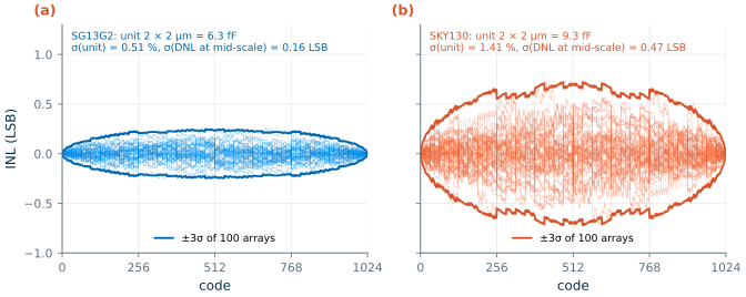
We checked Eq. (21.9) by simulating 100 arrays of 10 bits in each PDK, each unit a separate 2 µm × 2 µm MIM capacitor with the PDK’s mismatch model, so that every unit draws its own random error. An AC simulation measured every bit capacitor, and Eqs. (21.4)–(21.5) gave the DNL and INL. Figure 21.2 shows the result. The unit capacitors, 6.3 fF in SG13G2 and 9.3 fF in SKY130, have σu = 0.51 % and 1.41 %, which is Eq. (21.8) for 4 µm². At mid-scale σ(DNL) is 0.16 LSB in SG13G2 and 0.47 LSB in SKY130, against 0.16 and 0.45 LSB from Eq. (21.9); σ(INL) is 0.08 and 0.23 LSB. One SKY130 array in a hundred has a missing code.
For a DNL below ½ LSB at 3σ, Eq. (21.9) asks for \(\sigma_u < 0.5/(3\sqrt{2^N-1})\): 0.52 % at 10 bits, 0.26 % at 12 bits. With Eq. (21.8), a 10-bit DAC needs units of at least 3.8 µm² in SG13G2 but 30 µm² in SKY130; a 12-bit DAC needs 15 µm² and 118 µm². The kT/C noise of Section 18.7 would allow far smaller arrays: 0.58 pF in total for 12 bits over a 1.2 V range, where matching asks for 4096 units of 15 µm², 94 pF in SG13G2.
SG13G2 vs SKY130 · MIM capacitor matching
The SG13G2 MIM capacitor matches 2.8 times better than the SKY130 one for the same area, so it needs eight times less area for the same linearity. SKY130’s capacitor, with its 2 fF/µm², packs more capacitance per area, but for a DAC limited by matching that does not help. Above about 10 bits, designers stop paying for matching with area and calibrate instead: they measure each capacitor’s error, with the converter itself, and correct it digitally or with small trim capacitors.
21.6 ADC architectures
ADCs differ in how many comparisons they make at once [65, 52]:
- A flash ADC compares the input with all \(2^N - 1\) levels of a resistor string at once, with \(2^N - 1\) comparators, and converts the resulting thermometer code to binary. One clock period per sample makes it the fastest, but the number of comparators doubles with every bit, and each needs an offset well below an LSB: with the 8 mV offset of Chapter 20, 6 bits over 1.2 V is already difficult.
- A successive-approximation (SAR) ADC finds the code by binary search: one comparator, a DAC and a register take \(N\) decisions per sample. Its circuits are capacitors, switches, a latch and logic, so it gains from every new process, and it dominates the medium-resolution, medium-speed range at the lowest energy [113].
- A pipelined ADC splits the conversion over a chain of stages. Each stage resolves a few bits with a small flash ADC, subtracts the result from its input with a DAC and amplifies the remainder, the residue, for the next stage with a switched-capacitor gain stage (Section 18.6) [93]. All stages work at once on successive samples, so it converts one sample per clock period at high resolution, at the price of accurate amplifiers.
- A delta-sigma (ΔΣ) ADC samples far faster than the signal requires and puts a coarse quantizer, often of one bit, in a feedback loop that shapes the quantization noise away from the signal band [109, 66]. A digital filter removes the noise outside the band.
Oversampling and noise shaping
If the quantization noise of Eq. (21.2) is white, sampling at \(f_s = 2\,\mathrm{OSR}\,f_B\) for a signal band \(f_B\) leaves only a fraction 1/OSR of it in the band: each doubling of the oversampling ratio OSR gains 3 dB, half a bit. A ΔΣ modulator does much better by placing the quantizer after a loop filter of order \(L\) (a chain of \(L\) integrators) inside a feedback loop. The loop forces the average of the output to follow the input, and the quantization noise reaches the output shaped by \((1 - z^{-1})^L\), which is small at low frequencies and rises at \(20L\) dB per decade. In the signal band,
\[\mathrm{SQNR} = \mathrm{SQNR}_0 - 10\log_{10}\frac{\pi^{2L}}{2L+1} + (20L+10)\log_{10}\mathrm{OSR}, \tag{21.10}\]where \(\mathrm{SQNR}_0\) is the SQNR of the quantizer alone: each doubling of OSR gains \(6L + 3\) dB [66]. Figure 21.3 simulates first- and second-order modulators with a one-bit quantizer. The second-order loop follows the slope of Eq. (21.10), 15.0 dB per doubling, and reaches 99.7 dB at an OSR of 256, 3.6 dB below the linear model and about 16 bits from a one-bit quantizer. The first-order loop gains only 7.8 dB per doubling: its quantization error is far from random, and appears as idle tones in its spectrum, a reason why practical modulators are of second order or higher.
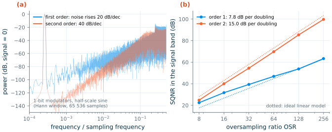
Table 21.1. The main ADC architectures. Typical ranges of published converters [13, 65].
| Architecture | Comparators | Clock periods per sample | Typical resolution | Typical sampling rate |
|---|---|---|---|---|
| Flash | \(2^N - 1\) | 1 | 4–8 bits | GS/s |
| SAR | 1 | about \(N\) | 8–16 bits | kS/s to hundreds of MS/s |
| Pipelined | a few per stage | 1 (with latency) | 10–16 bits | tens of MS/s to GS/s |
| Delta-sigma | 1 (or a few) | OSR per output sample | 12–24 bits | signal bands of Hz to tens of MHz |
21.7 A SAR ADC in both PDKs
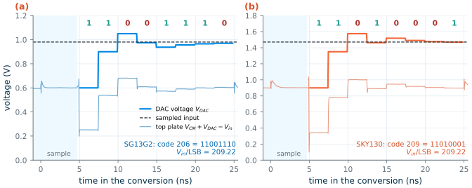
Figure 21.4 is the converter we simulate: an 8-bit charge-redistribution SAR ADC [110]. Its DAC is an array of binary-weighted MIM capacitors (128 to 1 units of 2 µm × 2 µm, plus a dummy unit: 1.62 pF in SG13G2 and 2.38 pF in SKY130), whose top plates connect to the inverting input of the StrongARM latch of Chapter 20. Each bottom plate has three switches: a transmission gate to the input, an NMOS to ground and a PMOS to \(V_{REF} = V_{DD}\), all sized in proportion to their capacitor so that every bit settles with the same time constant. The register that decides the bits is behavioural (ideal switches and controlled sources), so that the simulation contains every analog device but no logic gates.
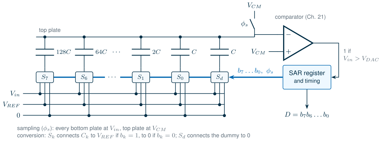
A conversion has two parts. During sampling (\(\phi_s\), two clock periods), the top plate is held at \(V_{CM} = V_{DD}/2\) and every bottom plate at \(V_{in}\), so the array stores the charge \(2^NC(V_{CM} - V_{in})\). The top-plate switch opens first, 0.2 ns before the bottom plates leave the input: this is the bottom-plate sampling of Section 19.4, which makes the charge injected by the top-plate switch independent of the input. During conversion the top plate floats, and when the bottom plates connect to the DAC voltage \(V_{DAC} = V_{REF}\sum_k b_k2^k/2^N\), charge conservation gives
\[V_{top} = V_{CM} + \left(V_{DAC} - V_{in}\right)\frac{2^NC}{2^NC + C_p}, \tag{21.11}\]where \(C_p\) is the parasitic capacitance of the top plate. The comparator only asks whether \(V_{top}\) is above or below \(V_{CM}\), so \(C_p\) attenuates the signal at its input but does not change the decision. The register first tries the MSB (\(V_{DAC} = V_{REF}/2\)). If the comparator finds \(V_{in} > V_{DAC}\) it keeps the bit, otherwise it clears it, and it tries the next bit; after eight decisions the bits are the code. The comparator runs at 400 MHz, and each bit has one clock period: the DAC settles while the latch resets, and the latch decides in the second half. With two periods of sampling, a conversion takes 25 ns: 40 MS/s.
Figure 21.5 shows one conversion in each PDK. The DAC voltage approaches the sampled input in halving steps, and the top plate mirrors it about \(V_{CM}\). The sample shown lies 209.2 LSB above zero in both PDKs. SKY130 converts it to 209 (11010001); SG13G2 to 206 (11001110), three codes lower because of the offset discussed below.
The demo below runs the same conversion one decision at a time: set the input, step or play the register’s eight trials, and add the simulated offset, a latch offset or comparator noise to see what each does to the code.
Spectrum, accuracy and energy
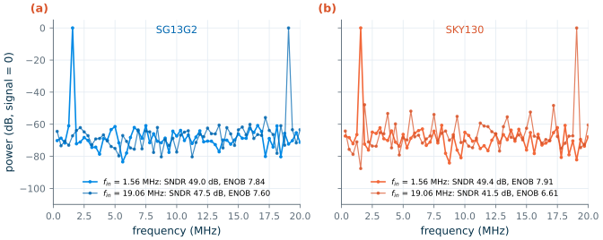
We converted 128 samples of a sine of 0.9 VDD peak to peak (−0.9 dBFS) in each PDK, at two input frequencies: 1.56 MHz, and 19.06 MHz, close to the Nyquist frequency of 20 MHz. Figure 21.6 shows the spectra of the codes. At low frequency the converter is close to ideal: SNDR = 49.0 dB in SG13G2 and 49.4 dB in SKY130, an ENOB of 7.84 and 7.91 bits, against 49.9 dB and 8 bits for an ideal 8-bit quantizer. Near Nyquist the SNDR falls to 47.5 dB in SG13G2 and 41.5 dB in SKY130, because the harmonics rise: the SFDR drops from 60.8 to 55.8 dB in SG13G2 and from 60.7 to 47.9 dB in SKY130. The cause is the input transmission gates. Their on-resistance changes with the signal, and the tracking error of Eq. (19.2) grows with the input frequency, as Section 19.2 predicted. SKY130 suffers more (THD −42.3 dB against −52.7 dB): with the same switch widths, its unit capacitors are 1.5 times larger and so is its input swing. Wider input switches, or a bootstrapped switch (Section 19.5), reduce the distortion.
A sine fit to the codes gives the static errors. The gain error is below 0.1 % in both PDKs. The offset is −2.9 LSB in SG13G2 and +0.4 LSB in SKY130. When the 48/96 µm top-plate switch opens, its channel charge and its clock feedthrough step the top plate, by about +13 mV in SG13G2, and a higher top plate reads as a lower input. In SKY130 the contributions of the NMOS and the PMOS cancel better. Thanks to bottom-plate sampling the step does not depend on the input, so it is a pure offset, removed by a digital subtraction. The comparator’s own offset (Chapter 20) would add to it in the same way.
The energy per conversion has two parts. Switching the capacitor array draws 2.21 pJ from \(V_{REF}\) in SG13G2 and 6.20 pJ in SKY130; the comparator, which decides ten times per conversion (also during sampling, where the decisions are ignored), draws 0.65 and 1.22 pJ. At 40 MS/s the converter dissipates 114 µW in SG13G2 and 297 µW in SKY130, a Walden figure of merit (Eq. 21.7) of 12 and 31 fJ per conversion step at low input frequency. These numbers leave out the logic, the clock and the circuit that drives the input, so a complete converter would be worse. The array dominates: it is 2.4 pF in SKY130 at 1.8 V, more than matching or kT/C requires at 8 bits: by Eqs. (21.8) and (21.9), a unit of 1 µm² would give σ(DNL) = 0.16 LSB in SG13G2 and 0.45 LSB in SKY130. A smaller unit and a smarter switching sequence, such as the monotonic switching of a differential array, which never charges a capacitor only to discharge it again, cut the switching energy by about 80 % [112].
What this means for your design
A SAR ADC is mostly capacitors and switches, and its accuracy budget is easy to write down. The sampling switch sets the bandwidth and the distortion at high input frequencies (Chapter 19). The capacitor array sets the linearity through matching and the noise through kT/C; size the unit for whichever is larger, and no larger, since the array also sets the energy. The comparator must resolve half an LSB at the input of the last decision within the time allowed (Chapter 20), and its offset and the top-plate switch’s pedestal only shift the curve.
Table 21.2. The 8-bit SAR ADC of Figure 21.4 in both PDKs (simulated, tt, 27 °C, 40 MS/s, sine of −0.9 dBFS, 128 samples).
| SG13G2 | SKY130 | |
|---|---|---|
| Full scale, LSB | 1.2 V, 4.69 mV | 1.8 V, 7.03 mV |
| Unit capacitor, total array | 6.3 fF, 1.62 pF | 9.3 fF, 2.38 pF |
| SNDR, ENOB at 1.56 MHz | 49.0 dB, 7.84 | 49.4 dB, 7.91 |
| SFDR at 1.56 MHz | 60.8 dB | 60.7 dB |
| SNDR, ENOB at 19.06 MHz | 47.5 dB, 7.60 | 41.5 dB, 6.61 |
| SFDR at 19.06 MHz | 55.8 dB | 47.9 dB |
| Offset | −2.9 LSB | +0.4 LSB |
| Energy per conversion: DAC, comparator | 2.21 pJ, 0.65 pJ | 6.20 pJ, 1.22 pJ |
| Power, Walden FoM (1.56 MHz) | 114 µW, 12 fJ/step | 297 µW, 31 fJ/step |
Try it · The converter script
Every number in this chapter comes from
tools/figs/ch22_converters.py. Runpython3 tools/figs/ch22_converters.py quant dsmfor the behavioural figures (seconds),capmcfor the capacitor arrays (minutes; add--resimto simulate again instead of redrawing) andsar sky130:lofor one SAR simulation (about 20 minutes), thensarwave sarfft. Three experiments: (1) changeCUto 1 µm and runcapmc --resim: does σDNL double, as Eq. (21.8) says? (2) HalveWSW, the width of the input switches, and simulate the 19.06 MHz input: how much SFDR do you lose? (3) Infig_quant, quantize a sine of 64 cycles in 4096 samples instead of 67: what happens to the spectrum, and why?
- Quantization alone limits an N-bit converter to an SQNR of 6.02N + 1.76 dB for a full-scale sine; real converters are measured by their ENOB, the resolution of an ideal converter with the same SNDR.
- Offset and gain error shift and tilt the transfer curve and are easy to calibrate; DNL and INL bend it. A DNL within ±½ LSB guarantees no missing codes and monotonicity.
- A binary-weighted capacitor DAC is worst at mid-scale: σ(DNL) ≈ √(2N−1) σu. With 2 µm × 2 µm MIM units, σu is 0.51 % in SG13G2 and 1.41 % in SKY130, enough for 10 bits in SG13G2 but not in SKY130.
- Flash converters are fastest, SAR converters the most energy-efficient at medium resolution, pipelined converters fast at high resolution, and delta-sigma converters trade speed for resolution by oversampling and noise shaping (6L + 3 dB per doubling of OSR).
- Our 8-bit, 40 MS/s SAR ADC reaches an ENOB of 7.84 (SG13G2) and 7.91 (SKY130) at low input frequency, for 2.9 and 7.4 pJ per conversion; near Nyquist, the distortion of the input switches costs 0.2 and 1.3 bits.
Further reading
- M. J. M. Pelgrom, Analog-to-Digital Conversion [65]: a complete textbook on sampling, quantization, DACs and every ADC architecture, by the author of the transistor matching law.
- J. L. McCreary and P. R. Gray [110]: the charge-redistribution SAR ADC, still the basis of most SAR converters; and B. Murmann [113] on why the SAR became the most versatile ADC.
- S. Pavan, R. Schreier and G. C. Temes, Understanding Delta-Sigma Data Converters [66]: the standard text on oversampling converters.
- R. H. Walden [96] and B. Murmann’s survey [13]: what the state of the art reaches, and the figures of merit used to compare it.
- BRICD, Open-BioAFE Tutorial: the next step. Its Part III picks up from this chapter with sampling, switches, comparators, capacitive DACs, the SAR ADC and ΔΣ converters, designed for an eight-channel biopotential front-end in IHP SG13G2.