Chapter 4
The MOSFET for Circuit Designers
A MOSFET is a voltage-controlled charge reservoir. Once you see it that way, the square law, its many corrections and the subthreshold region all follow from one picture.
- Explain inversion, threshold voltage and the operating regions of a MOSFET.
- Derive the square-law model and use it for hand calculations.
- Account for body effect, channel-length modulation and DIBL.
- Describe weak and moderate inversion and the short-channel effects of a 130 nm device.
- Judge how far the square law can be trusted, using SG13G2 and SKY130 simulations.
Contents
4.1 Structure and terminals
A MOSFET (metal-oxide-semiconductor field-effect transistor) is a capacitor whose bottom plate can conduct. Figure 4.1 shows the two kinds that every CMOS process offers. In the NMOS transistor, two heavily doped n-type regions, the source and the drain, sit in a p-type substrate. Between them, a thin layer of silicon dioxide, the gate oxide, separates the silicon from a conducting gate of doped polysilicon. The distance between source and drain under the gate is the channel length \(L\); the extent of the device into the page is its width \(W\). The PMOS transistor is the mirror image: p-type source and drain in an n-type well.
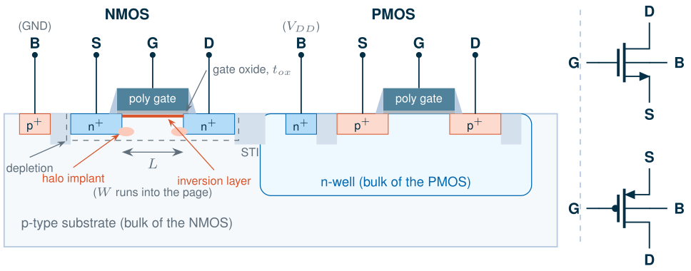
The device has four terminals. The gate (G) controls the channel; current flows between drain (D) and source (S); the bulk (B, also called body) is the silicon underneath. The structure is symmetric: the source is simply the terminal at the lower potential for an NMOS (higher for a PMOS), and it can swap with the drain during operation, for example in a switch. The bulk of every NMOS is the same substrate, so it is usually at ground for all of them; each PMOS sits in an n-well that can be tied to \(V_{DD}\) or to its own source. Section 4.4 shows what a bulk at a different potential from the source does.
Two details from the cross-section return later. The drawn length and width in the netlist are not the electrical ones: the source and drain diffuse a little under the gate, and the isolation eats into the width. For a device drawn 5 µm × 0.5 µm, the models report an effective length of 0.441 µm in SG13G2 and 0.476 µm in SKY130. And the small halo (or pocket) implants beside the source and drain, added to control short-channel effects, make the threshold voltage depend strongly on length (Section 4.6). If you want to see what a real transistor layout looks like, the PDK Devices in 3D gallery shows both PDKs’ MOSFETs extruded through their layer stacks.
In a netlist, a MOSFET is a subcircuit with its terminals in the order drain, gate, source, bulk. The core (thin-oxide) devices of the two PDKs are instantiated like this (Chapter 3 explains the model files):
* SG13G2 1.2 V core devices: W and L with units; ng = number of gate fingers
.lib cornerMOSlv.lib mos_tt
XMN d g s b sg13_lv_nmos W=5u L=0.5u ng=1 m=1
XMP d g s b sg13_lv_pmos W=5u L=0.5u ng=1 m=1
* SKY130 1.8 V core devices: W and L in um (the library sets .option scale=1.0u); nf = fingers
.lib "$PDK_ROOT/sky130A/libs.tech/ngspice/sky130.lib.spice" tt
XMN d g s b sky130_fd_pr__nfet_01v8 W=5 L=0.5 nf=1 ad=1.45 as=1.45 pd=10.58 ps=10.58 mult=1 m=1
XMP d g s b sky130_fd_pr__pfet_01v8 W=5 L=0.5 nf=1 ad=1.45 as=1.45 pd=10.58 ps=10.58 mult=1 m=1
SG13G2 vs SKY130 · The core transistors
The SG13G2 core devices are built for a 1.2 V supply, with a minimum length of 0.13 µm and a gate oxide about 2.45 nm thick [15]. The SKY130 core devices are 1.8 V transistors with a minimum length of 0.15 µm and a 4.1 nm oxide [19, 18]. SG13G2 is modelled with PSP, a surface-potential model [73]; SKY130 with BSIM4. Both PDKs also offer thick-oxide devices for 3.3 V (SG13G2) and 5 V (SKY130) that this chapter does not cover. Throughout the chapter every transistor is 5 µm wide, the width of the lookup tables in Chapter 6.
4.2 Threshold and inversion
Think of the gate and the silicon as the two plates of a capacitor with the oxide as dielectric. Its capacitance per unit area is
\[C_{ox} = \frac{\varepsilon_{ox}}{t_{ox}}, \qquad \varepsilon_{ox} = 3.9\,\varepsilon_0 = 34.5\ \mathrm{aF/\mu m}. \tag{4.1}\]For the SG13G2 oxide of 2.45 nm this gives 14.1 fF/µm²; for the 4.1 nm SKY130 oxide, 8.4 fF/µm². What changes as we raise the gate voltage of an NMOS is the charge on the silicon plate.
- Accumulation (\(V_{GS}\) well below zero). The negative gate attracts holes, the majority carriers of the p-type substrate, to the surface. The silicon plate is a good conductor and the capacitance is close to \(C_{ox}\).
- Depletion (around zero to a few hundred millivolts). The positive gate pushes the holes away and leaves behind a layer of fixed, negatively charged acceptor ions. This depletion region adds its own capacitance in series with the oxide, so the total falls.
- Inversion (above the threshold). The surface potential has risen so far that electrons, the minority carriers, gather in a thin layer at the surface: the inversion layer, or channel. It connects source and drain, and every extra volt on the gate adds \(C_{ox}\) worth of electrons to it.
The threshold voltage \(V_{TH}\) is the gate voltage at which inversion sets in. In the classic textbook definition it is the voltage at which the surface electron density equals the bulk hole density, which happens when the surface potential reaches \(2\phi_F\), twice the Fermi potential of the substrate [58, 51]:
\[V_{TH} = V_{FB} + 2\phi_F + \gamma\sqrt{2\phi_F}, \qquad \gamma = \frac{\sqrt{2q\varepsilon_{si}N_A}}{C_{ox}}. \tag{4.2}\]\(V_{FB}\), the flat-band voltage, accounts for the work-function difference between gate and silicon; the last term is the voltage needed to hold the depletion charge. Above threshold, the inversion charge per unit area grows linearly with gate voltage:
\[Q_{inv} = -C_{ox}\,(V_{GS} - V_{TH}). \tag{4.3}\]This is the single most useful idea in the chapter: the gate voltage above threshold, the overdrive \(V_{OV} = V_{GS} - V_{TH}\), sets how much mobile charge the channel holds. Everything else follows from asking how fast that charge moves.
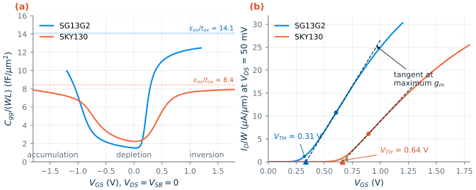
Figure 4.2(a) shows the three regions in simulation. It plots the intrinsic gate capacitance per unit area of a long NMOS (W/L = 5/2) with source, drain and bulk grounded, as ngspice computes it from each PDK’s model. Strong inversion gives 12.5 fF/µm² in SG13G2 and 7.9 fF/µm² in SKY130, 11 % and 6 % below Eq. (4.1). The difference is real physics, not a modelling error: the polysilicon gate is itself slightly depleted, and the electrons in the channel sit a fraction of a nanometre below the surface. Both effects add to the oxide thickness, so the electrical thickness is 2.77 nm and 4.36 nm. For hand calculations, use the inversion value.
Measuring the threshold
\(V_{TH}\) is not a terminal quantity that a voltmeter can read, so it has to be extracted from a current measurement, and different methods give different answers. The most common one for circuit work, used throughout this book, is linear extrapolation: bias the drain at a small voltage (50 mV) so that the device behaves as a resistor, sweep the gate, find the point of maximum transconductance \(g_m = \partial I_D/\partial V_{GS}\), and extend the tangent there down to zero current. Its intercept, minus half the drain voltage, is \(V_{TH}\). Figure 4.2(b) shows the construction for W/L = 5/0.5. It gives 0.31 V for SG13G2 and 0.64 V for SKY130. In ngspice the whole extraction takes five lines of .control code:
* Threshold by linear extrapolation, SG13G2 NMOS W/L = 5/0.5
.lib cornerMOSlv.lib mos_tt
Vd d 0 0.05
Vg g 0 0
XM1 d g 0 0 sg13_lv_nmos W=5u L=0.5u ng=1 m=1
.control
dc vg 0 1.2 0.005
let id = -i(vd)
let gm = deriv(id)
meas dc gmmax max gm
meas dc vgm max_at gm
meas dc idm find id at=vgm
let vth = vgm - idm/gmmax - 0.025
print vth                  $ 0.311 V
.endc
.end
* Threshold by linear extrapolation, SKY130 NMOS W/L = 5/0.5
.lib "$PDK_ROOT/sky130A/libs.tech/ngspice/sky130.lib.spice" tt
Vd d 0 0.05
Vg g 0 0
XM1 d g 0 0 sky130_fd_pr__nfet_01v8 W=5 L=0.5 nf=1
.control
dc vg 0 1.8 0.005
let id = -i(vd)
let gm = deriv(id)
meas dc gmmax max gm
meas dc vgm max_at gm
meas dc idm find id at=vgm
let vth = vgm - idm/gmmax - 0.025
print vth                  $ 0.638 V
.endc
.end
Common pitfall · Treating VTH as a single, exact number
The models also report a threshold as an operating-point value (
vth), computed by their own internal definitions. For the same 5/0.5 devices it is 0.27 V in SG13G2 and 0.63 V in SKY130: 40 mV and 10 mV below the extrapolated values. A constant-current definition (the gate voltage at which \(I_D = 100\ \mathrm{nA}\cdot W/L\)) gives yet another number. None of them is wrong; they are different definitions. Always say which one you used, and never mix a \(V_{TH}\) from one method with a \(\mu C_{ox}\) fitted with another (Section 4.7).
4.3 The square-law model
Now let the charge move. With a drain voltage applied, the channel potential \(V(x)\) rises from 0 at the source to \(V_{DS}\) at the drain, so the local overdrive, and with it the local channel charge, falls along the channel: \(Q_{inv}(x) = -C_{ox}\,(V_{GS} - V_{TH} - V(x))\). The electrons drift in the lateral field with a velocity \(v = \mu_n\,dV/dx\), where \(\mu_n\) is the electron mobility in the channel. The current is charge per unit length times velocity, and it must be the same at every point:
\[I_D = W\,C_{ox}\,(V_{GS} - V_{TH} - V(x))\;\mu_n\frac{dV}{dx}.\]Integrating from source to drain gives the triode (or linear) region current,
\[I_D = \mu_n C_{ox}\frac{W}{L}\Big[(V_{GS}-V_{TH})V_{DS} - \tfrac{1}{2}V_{DS}^2\Big], \qquad V_{DS} < V_{GS}-V_{TH}. \tag{4.4}\]For small \(V_{DS}\) the device is a resistor, \(R_{on} = 1/\big(\mu_n C_{ox}(W/L)V_{OV}\big)\), which is how a MOSFET switch is used. As \(V_{DS}\) rises, the channel charge at the drain end falls, until at \(V_{DS} = V_{OV}\) it reaches zero: the channel is pinched off. Beyond this point the extra drain voltage drops across a short depleted region next to the drain, and the current stops growing. This is the saturation region, where amplifying transistors are biased.
Key equation · The square law in saturation
\[I_D = \tfrac{1}{2}\mu_n C_{ox}\frac{W}{L}\,(V_{GS}-V_{TH})^2, \qquad V_{DS} \geq V_{DS,sat} = V_{GS}-V_{TH}. \tag{4.5}\]For a PMOS, use \(\mu_p\) and the magnitudes \(\lvert V_{GS}\rvert\), \(\lvert V_{TH}\rvert\), \(\lvert V_{DS}\rvert\). The product \(\mu C_{ox}\) is often written \(k'\), the process transconductance parameter.
Derivation · From the charge sheet to Eqs. (4.4) and (4.5)
Start from the current at a point \(x\) in the channel, which is constant along the channel:
\[I_D = \mu_n W C_{ox}\,(V_{GS} - V_{TH} - V)\,\frac{dV}{dx}.\]Separate the variables and integrate \(x\) from 0 to \(L\) and \(V\) from 0 to \(V_{DS}\):
\[\int_0^L I_D\,dx = \mu_n W C_{ox}\int_0^{V_{DS}} (V_{GS} - V_{TH} - V)\,dV \;\;\Rightarrow\;\; I_D L = \mu_n W C_{ox}\Big[(V_{GS}-V_{TH})V_{DS} - \tfrac{1}{2}V_{DS}^2\Big],\]which is Eq. (4.4). It is a parabola in \(V_{DS}\) with its maximum at \(V_{DS} = V_{GS}-V_{TH}\), where \(\partial I_D/\partial V_{DS} = 0\). That maximum is where the charge at the drain end, \(C_{ox}(V_{GS}-V_{TH}-V_{DS})\), vanishes. Beyond it the equation no longer applies (it would predict a falling current); physically the pinch-off point simply holds the channel potential at \(V_{OV}\), so the current stays at its peak value. Substituting \(V_{DS} = V_{OV}\) gives Eq. (4.5).
Two approximations hide in this derivation. First, \(V_{TH}\) was taken as constant along the channel, but the depletion charge under the channel grows as \(V(x)\) rises, which raises the local threshold. Including it divides the saturation current and \(V_{DS,sat}\) by the slope factor \(n \approx 1.2\)–1.5 of Section 4.5, \(I_D = \mu_n C_{ox}(W/L)V_{OV}^2/(2n)\) [58, 59]. Second, \(\mu_n\) was taken as constant, which Section 4.6 corrects. Both are absorbed into the fitted \(\mu C_{ox}\) when we fit the square law to a real device in Section 4.7.
This model goes back to Shichman and Hodges [71], and it is still the starting point of every analog textbook [51, 52, 53]. Figure 4.3 shows how well its shape matches the output characteristics, \(I_D\) against \(V_{DS}\), of the two 5/0.5 NMOS devices, for overdrives of 0.1 to 0.5 V above the extracted threshold.
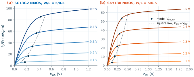
The shape is right: a linear rise, a knee and a nearly flat saturation region. Three details are not.
- At the same overdrive, SG13G2 delivers more current, 99 µA/µm against 64 µA/µm at \(V_{OV} = 0.5\) V. Its thinner oxide holds more charge per volt (Figure 4.2a).
- The knee is not at \(V_{DS} = V_{OV}\). At small overdrive the device saturates later than predicted (the model gives 0.17 V and 0.12 V at \(V_{OV} = 0.1\) V), because near threshold the current saturates only after a few thermal voltages, \(V_{DS} \approx 4U_T\) (Section 4.5). At large overdrive it saturates earlier (0.42 V and 0.35 V at \(V_{OV} = 0.5\) V), because the carriers reach their maximum velocity before the channel pinches off (Section 4.6).
- The current in saturation is not flat. That slope is the subject of the next section, and it limits the gain of every amplifier in this book.
4.4 Body effect, channel-length modulation and DIBL
The square law depends on two voltages, \(V_{GS}\) and, in triode, \(V_{DS}\). A real transistor also responds to the bulk voltage and, in saturation, to the drain voltage. These second-order effects decide the gain of amplifiers and the accuracy of current mirrors.
Body effect
If the source sits above the bulk, \(V_{SB} > 0\) (common in stacked transistors, such as cascodes and the input pair of a differential amplifier), the reverse-biased source junction widens the depletion region under the channel. More depletion charge must now be supported by the gate before inversion starts, so the threshold rises. Replacing \(2\phi_F\) by \(2\phi_F + V_{SB}\) in the depletion term of Eq. (4.2) gives
\[V_{TH} = V_{TH0} + \gamma\Big(\sqrt{2\phi_F + V_{SB}} - \sqrt{2\phi_F}\Big), \tag{4.6}\]where \(V_{TH0}\) is the threshold at \(V_{SB} = 0\) and \(\gamma\) is the body-effect coefficient of Eq. (4.2). The square root means the effect is strongest for the first few hundred millivolts of \(V_{SB}\).
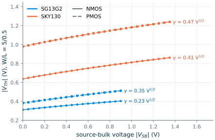
Figure 4.4 shows the extracted threshold (linear extrapolation, \(V_{DS}\) = 50 mV) against \(V_{SB}\) for both device types, with Eq. (4.6) fitted to each curve. The fits give \(\gamma\) = 0.23 V½ (NMOS) and 0.35 V½ (PMOS) in SG13G2, and 0.41 V½ and 0.47 V½ in SKY130, with \(2\phi_F\) between 0.85 and 1.03 V. The thinner SG13G2 oxide (larger \(C_{ox}\)) explains most of the difference, since \(\gamma \propto 1/C_{ox}\). In numbers: raising the source of an NMOS by 0.5 V raises its threshold by 56 mV in SG13G2 and by 95 mV in SKY130.
Channel-length modulation
In saturation, a higher drain voltage widens the pinched-off region at the drain end, so the effective channel gets a little shorter and the current a little larger. The first-order model multiplies Eq. (4.5) by a linear factor:
\[I_D = \tfrac{1}{2}\mu_n C_{ox}\frac{W}{L}V_{OV}^2\,(1 + \lambda V_{DS}), \qquad \lambda = \frac{1}{V_A}. \tag{4.7}\]\(V_A\) is the Early voltage, by analogy with the bipolar transistor: extrapolate the saturated output curves backwards and they meet the \(V_{DS}\) axis near \(-V_A\). The small-signal output resistance is then \(r_o \approx V_A/I_D\) (Chapter 5). Because the pinch-off region is a fixed fraction of a short channel but a tiny fraction of a long one, \(V_A\) grows roughly in proportion to \(L\).
Drain-induced barrier lowering
In a short device the drain is close enough to the source to help the gate: its field lowers the potential barrier that electrons must climb to leave the source. The threshold then falls as \(V_{DS}\) rises, which is drain-induced barrier lowering (DIBL), usually described by a coefficient \(\eta\) in mV of threshold shift per volt of drain voltage:
\[V_{TH} = V_{TH0} - \eta\,V_{DS}. \tag{4.8}\]A falling threshold raises the current, so DIBL adds to the output conductance. In modern short devices it is often the larger of the two effects.
Figure 4.5 measures both. Panel (a) plots \(V_A = I_D/g_{ds}\) against length at a fixed overdrive of 0.2 V and \(V_{DS} = V_{DD}/2\). Panel (b) plots the threshold shift against \(V_{DS}\), using the constant-current definition (which works at any drain voltage).
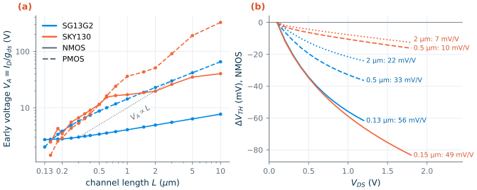
At minimum length the two processes are alike: an Early voltage of about 2.5 V and a DIBL of about 50 mV/V (56 mV/V in SG13G2, 49 mV/V in SKY130). With length they part ways. The SKY130 NMOS behaves as the textbook says: \(V_A\) rises from 2.5 V at 0.15 µm to 11.5 V at 0.5 µm and 20 V at 2 µm, and DIBL falls to 10 and 7 mV/V. The SG13G2 NMOS barely improves: its \(V_A\) is 3.4 V at 0.5 µm, 4.9 V at 2 µm and only 7.7 V at 10 µm, and its DIBL is still 22 mV/V at 2 µm. The PMOS devices of both processes scale with length (SG13G2: 8.7 V at 0.5 µm, 23 V at 2 µm).
SG13G2 vs SKY130 · Why the SG13G2 NMOS has so little output resistance
In a long, uniformly doped transistor the drain has almost no influence on the threshold. The SG13G2 NMOS is not uniformly doped: the strong rise of its threshold at short lengths (Figure 4.7a) is the signature of heavy halo implants at both ends of the channel [58]. The drain voltage lowers the barrier of the drain-side halo even when the channel is long, so the device keeps a drain-induced threshold shift of about 20 mV/V even at lengths of 2 µm and more. This is why the SG13G2 NMOS has 3 to 5 times less intrinsic gain than the SKY130 NMOS (Chapter 6). In SG13G2, a longer channel alone will not give you a high-impedance NMOS current source; use a cascode (Chapter 7) or a PMOS.
The demo below puts Sections 4.2 to 4.4 into one cross-section: move \(V_{GS}\), \(V_{DS}\) and \(V_{SB}\), or pick an effect, and watch the holes, the depletion region, the electron sheet and the source barrier respond, with the threshold and the current read from the simulations above and the tables of Chapter 6.
The drawing is qualitative: charges, depletion widths and the band are scaled for visibility. Every number comes from the chapter's simulations or the gm/ID tables.
4.5 Weak and moderate inversion
The square law says a transistor carries no current below threshold. Figure 4.6 shows that this is only true on a linear scale. On a logarithmic scale (panel a), the current below threshold falls by a constant factor for every millivolt of gate voltage: it is exponential, over six or seven decades.
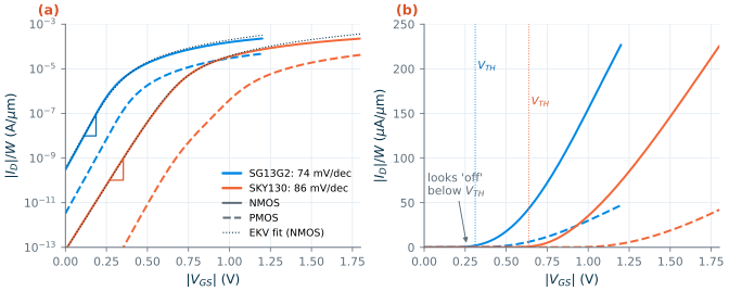
Below threshold there is too little charge in the channel for drift to matter. Instead, electrons diffuse from the source, where their density is high, to the drain, where the drain voltage has removed them, just as the carriers do in the base of a bipolar transistor. The number of electrons that can get over the source barrier depends exponentially on the surface potential, and the gate controls the surface potential through a capacitive divider: the oxide capacitance in series with the depletion capacitance \(C_{dep}\). Only a fraction \(1/n\) of a gate-voltage change reaches the surface, where \(n = 1 + C_{dep}/C_{ox}\) is the slope factor. The result is [58, 59]
\[I_D = I_0\,\frac{W}{L}\,\exp\!\left(\frac{V_{GS}-V_{TH}}{nU_T}\right)\left[1 - \exp\!\left(-\frac{V_{DS}}{U_T}\right)\right], \tag{4.9}\]with \(U_T = kT/q = 25.9\) mV at 27 °C and \(I_0\) a process constant. The drain term saturates after \(V_{DS} \approx 4U_T \approx 100\) mV, so a weakly inverted transistor stays in saturation down to very low drain voltages. A useful figure of merit is the gate-voltage change needed for a tenfold change in current, the subthreshold slope:
\[S = \frac{dV_{GS}}{d\log_{10} I_D} = n\,U_T\ln 10 \approx n \cdot 59.5\ \mathrm{mV/decade}. \tag{4.10}\]An ideal device (\(n = 1\)) would need 59.5 mV per decade at room temperature. The simulated NMOS devices of Figure 4.6 need 74 mV/decade in SG13G2 (\(n\) = 1.24) and 86 mV/decade in SKY130 (\(n\) = 1.44). Table 4.1 lists the slope for three lengths and both device types.
Table 4.1. Subthreshold slope S (mV/decade) and slope factor n, at |VDS| = VDD/2, W = 5 µm, 27 °C.
| Device | SG13G2 Lmin | SG13G2 0.5 µm | SG13G2 2 µm | SKY130 Lmin | SKY130 0.5 µm | SKY130 2 µm |
|---|---|---|---|---|---|---|
| NMOS, S | 83 | 74 | 73 | 95 | 86 | 86 |
| NMOS, n | 1.39 | 1.24 | 1.22 | 1.59 | 1.44 | 1.45 |
| PMOS, S | 86 | 74 | 72 | 106 | 79 | 77 |
| PMOS, n | 1.45 | 1.25 | 1.22 | 1.79 | 1.33 | 1.30 |
Two consequences matter for design. First, a transistor at \(V_{GS} = 0\) is not off. At \(V_{DS} = V_{DD}/2\) the SG13G2 NMOS (L = 0.5 µm) still leaks 300 pA per micrometre of width, because its threshold is low; the SKY130 NMOS leaks 75 fA/µm. Second, the exponential law gives the largest transconductance per unit current a MOSFET can reach, \(g_m/I_D = 1/(nU_T)\), which is the basis of the \(g_m/I_D\) method of Chapter 6.
Moderate inversion and a model for all regions
Between the exponential and the square-law regions lies moderate inversion, where drift and diffusion both carry current. Neither Eq. (4.5) nor Eq. (4.9) describes it, yet it is where many low-power analog transistors are biased. The EKV model [72, 59] joins the two regions with one smooth expression. In saturation, referred to the source,
\[I_D = I_S\,\ln^2\!\left[1 + \exp\!\left(\frac{V_{GS}-V_{TH}}{2nU_T}\right)\right], \qquad I_S = 2n\,\mu C_{ox}\frac{W}{L}\,U_T^2. \tag{4.11}\]Far below threshold, \(\ln(1+e^x) \approx e^x\) and Eq. (4.11) becomes the exponential of Eq. (4.9). Far above threshold, \(\ln(1+e^x) \approx x\) and it becomes \(\mu C_{ox}(W/L)V_{OV}^2/(2n)\), the square law with the slope factor of the derivation box. The dotted lines in Figure 4.6(a) fit Eq. (4.11) to each NMOS with \(n\) fixed at its measured value and only \(V_{TH}\) and \(I_S\) adjusted: one expression follows the simulation over nine decades of current. Chapter 6 uses the same model to define the inversion coefficient.
4.6 Short-channel effects at 130 nm
The square law assumes a long channel: a constant mobility, a carrier velocity proportional to the field, and a threshold set by the doping alone. At 130 nm all three assumptions break.
Velocity saturation
The carrier velocity \(v = \mu E\) cannot grow without bound. Above a lateral field of a few volts per micrometre the electrons scatter off the crystal lattice so often that their velocity saturates at \(v_{sat} \approx 10^7\) cm/s [58]. With 0.5 V across a 0.13 µm channel the average field is already almost 4 V/µm. A common way to include this in the square law is to divide by a factor that grows with the field [51, 52]:
\[I_D = \frac{\tfrac{1}{2}\mu_n C_{ox}(W/L)\,V_{OV}^2}{1 + V_{OV}/(E_c L)}, \qquad E_c = \frac{2v_{sat}}{\mu_n}. \tag{4.12}\]For a long channel (\(V_{OV} \ll E_cL\)) this is the square law. For a short one (\(V_{OV} \gg E_cL\)) it becomes \(I_D \approx \tfrac{1}{2}WC_{ox}v_{sat}V_{OV}\): linear in overdrive, and independent of length. The transconductance then stops growing with overdrive and saturates at \(g_m \approx W C_{ox} v_{sat}\).
Mobility degradation
Even in a long channel, the vertical field of the gate pulls the electrons against the oxide interface, where they scatter more. The mobility falls as the overdrive rises, often modelled as
\[\mu_{eff} = \frac{\mu_0}{1 + \theta V_{OV}}, \tag{4.13}\]with a fitting parameter \(\theta\) of a few tenths per volt. Its effect looks like a mild velocity saturation: the current grows more slowly than \(V_{OV}^2\) at high overdrive.
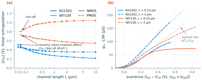
Figure 4.7(b) separates the two effects. It plots \(g_m L/W\) against overdrive in saturation. For an ideal square-law device this is a straight line of slope \(\mu C_{ox}\), the same for every length (the dotted lines, fitted in Section 4.7). The 2 µm SKY130 device follows the line up to about 0.35 V of overdrive and then bends below it: mobility degradation (the SG13G2 device stays on its line over the smaller range that its 1.2 V supply allows). The minimum-length devices bend over much earlier and flatten at about 97 µS (SG13G2) and 74 µS (SKY130): velocity saturation. Their transconductance per micrometre of width peaks at 0.81 mS/µm and 0.49 mS/µm, against the hand estimate \(C_{ox}v_{sat}\) = 12.5 fF/µm² × 10⁵ m/s = 1.25 mS/µm and 0.79 mS/µm. The estimate is high by 50 to 60 %, as expected from such a crude model, but it predicts the right order of magnitude and the right ratio between the two processes.
Threshold versus length
In a uniformly doped device, a shorter channel has a lower threshold: the source and drain junctions deplete part of the region under the gate themselves, so the gate has less charge to support. This is threshold roll-off. To fight it, modern processes add the halo implants of Figure 4.1, which raise the doping next to the source and drain. In a short device the halos cover a large fraction of the channel, so the threshold rises at short lengths. This is the reverse short-channel effect (RSCE) [58].
Figure 4.7(a) shows that both NMOS devices are dominated by RSCE. The SG13G2 NMOS threshold rises from 0.23 V at 5 µm to 0.31 V at 0.5 µm and 0.52 V at 0.13 µm, a 290 mV change; the SKY130 NMOS rises from 0.55 V to 0.64 V and 0.72 V. The SG13G2 PMOS shows a milder RSCE (0.35 to 0.46 V). The SKY130 PMOS is the odd one out: its threshold falls from 1.04 V at 5 µm to 0.81 V at 0.15 µm, the classic roll-off.
What this means for your design
Do not reuse a threshold across lengths. A current mirror with a 0.13 µm reference device and a 0.5 µm output device in SG13G2 has 200 mV of threshold difference built in. Keep matched devices at the same length, and when you change L in a design, look up the new \(V_{GS}\) instead of assuming it. Short devices also bring velocity saturation (less \(g_m\) per unit current at high overdrive) and DIBL (less gain). Minimum length is for switches and digital gates; analog transistors usually start at two to four times \(L_{min}\) (Chapter 6, Section 6.7).
4.7 How good is the square law?
Every hand calculation in the following chapters starts from Eq. (4.5), so it is worth knowing how far to trust it. The test is simple: fit the square law to a simulated device, then compare. Taking the square root of Eq. (4.5),
\[\sqrt{I_D} = \sqrt{\tfrac{1}{2}\mu C_{ox}\tfrac{W}{L}}\;(V_{GS} - V_{TH}),\]so \(\sqrt{I_D}\) against \(V_{GS}\) should be a straight line. Its slope gives \(\mu C_{ox}\) and its intercept gives \(V_{TH}\). We fit the line by least squares over \(V_{GS}\) from 0.1 to 0.4 V above the extracted threshold, at \(\lvert V_{DS}\rvert = V_{DD}/2\), the range of overdrive in which analog transistors are typically biased. Table 4.2 lists the results.
Table 4.2. Square-law parameters fitted to simulation (saturation, |VDS| = VDD/2, W = 5 µm, tt, 27 °C). Use each pair together.
| Device and length | SG13G2 µCox (µA/V²) | SG13G2 VTH (V) | SKY130 µCox (µA/V²) | SKY130 VTH (V) |
|---|---|---|---|---|
| NMOS, Lmin | 192 | 0.42 | 172 | 0.61 |
| NMOS, 0.5 µm | 286 | 0.25 | 215 | 0.59 |
| NMOS, 2 µm | 315 | 0.20 | 233 | 0.54 |
| NMOS, 5 µm | 320 | 0.18 | 224 | 0.52 |
| PMOS, Lmin | 74 | 0.39 | 46 | 0.66 |
| PMOS, 0.5 µm | 70 | 0.34 | 60 | 0.94 |
| PMOS, 2 µm | 73 | 0.33 | 61 | 1.00 |
| Body effect γ, NMOS / PMOS (V½) | 0.23 / 0.35 | 0.41 / 0.47 | ||
| Inversion Cox (fF/µm²) | 12.5 | 7.9 |
A few things stand out. The NMOS-to-PMOS ratio of \(\mu C_{ox}\) is 4.3 in SG13G2 and 3.8 in SKY130, so a PMOS must be about four times wider than an NMOS for the same current. For lengths of 0.5 µm and more, the fitted thresholds are 30 to 60 mV below the extrapolated ones of Section 4.2, because the fit absorbs part of the moderate-inversion current. And \(\mu C_{ox}\) falls at short lengths, by 40 % at \(L_{min}\) in SG13G2: velocity saturation, absorbed into the fit. Dividing by the inversion capacitance gives effective electron mobilities of about 250 cm²/Vs (SG13G2) and 290 cm²/Vs (SKY130) at 2 µm, about a fifth of the mobility in bulk silicon, because of the interface scattering of Section 4.6.
Figure 4.8 shows how good the fit is. On a linear scale (panel a) the square law and the simulation are hard to tell apart near the fitting window, and only part company at high gate voltage. Panel (b) shows the ratio of the two over the whole range of overdrive.
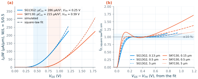
The square law is within 10 % of the simulation between about 0.15 and 0.6 V of overdrive at every length (from 0.2 V for the minimum-length SKY130 device), and up to 0.7 to 1 V of overdrive for lengths of 0.5 µm and more. Outside that band it fails in both directions.
- Near threshold it underestimates. At 50 mV of overdrive it predicts less than half the real current (ratios of 0.46 for SG13G2 and 0.55 for SKY130 at L = 0.5 µm), and below threshold it predicts nothing at all. This is moderate and weak inversion, where Section 4.5 applies.
- At high overdrive it overestimates, because of mobility degradation and velocity saturation. At \(V_{GS} = V_{DD}\) the ratio reaches 1.14 for the SG13G2 device of 0.5 µm and 1.39 for the SKY130 one; for the minimum-length SKY130 device it is 1.71.
- The fitted parameters only hold near the device they were fitted to. Change L, and both \(\mu C_{ox}\) and \(V_{TH}\) move (Table 4.2).
The worked example puts numbers on all three points.
Worked example 4.1 · Biasing an NMOS at 50 µA
An NMOS with W/L = 5 µm/0.5 µm, source and bulk grounded, must carry \(I_D\) = 50 µA in saturation. Find \(V_{GS}\) and \(V_{DS,sat}\) by hand, then \(V_{GS}\) when the source is raised to \(V_{SB}\) = 0.3 V, and finally \(V_{GS}\) for a minimum-length device of the same width.
Overdrive. From Eq. (4.5) with the 0.5 µm parameters of Table 4.2, \(V_{OV} = \sqrt{2I_D/(\mu C_{ox}\,W/L)}\). SG13G2: \(\sqrt{2 \cdot 50\ \mu\mathrm{A}/(286\ \mu\mathrm{A/V^2} \cdot 10)} = 0.187\) V. SKY130: \(\sqrt{2 \cdot 50/(215 \cdot 10)} = 0.216\) V.
Gate voltage. \(V_{GS} = V_{TH} + V_{OV}\) = 0.249 + 0.187 = 0.436 V (SG13G2) and 0.595 + 0.216 = 0.810 V (SKY130). The square law also predicts \(V_{DS,sat} = V_{OV}\) = 0.187 V and 0.216 V.
Body effect. With \(V_{SB}\) = 0.3 V, Eq. (4.6) with \(\gamma\) = 0.23 V½, \(2\phi_F\) = 0.85 V (SG13G2) gives \(\Delta V_{TH} = 0.23(\sqrt{1.15} - \sqrt{0.85}) = 35\) mV; with \(\gamma\) = 0.41 V½, \(2\phi_F\) = 0.95 V (SKY130), 59 mV. The gate must rise by the same amounts (at constant current, \(V_{OV}\) does not change).
Minimum length. Reusing the 0.5 µm parameters for W/L = 5/0.13 (SG13G2) gives \(V_{OV}\) = 0.095 V and \(V_{GS}\) = 0.344 V; for 5/0.15 (SKY130), 0.118 V and 0.713 V.
Simulation (ngspice, \(V_{DS} = V_{DD}/2\)):
Quantity SG13G2 hand SG13G2 sim SKY130 hand SKY130 sim \(V_{GS}\), L = 0.5 µm 0.436 V 0.434 V 0.810 V 0.811 V \(V_{DS,sat}\) 0.187 V 0.183 V 0.216 V 0.167 V \(\Delta V_{GS}\) for \(V_{SB}\) = 0.3 V 35 mV 35 mV 59 mV 59 mV \(V_{GS}\), \(L_{min}\) 0.344 V 0.516 V 0.713 V 0.754 V With parameters fitted to the device itself, the hand calculation is within 2 mV, and the body effect is exact. The saturation voltage is close in SG13G2 but 23 % high in SKY130, where the model saturates earlier. Moving the same parameters to the minimum length fails badly: 172 mV too low in SG13G2 (reverse short-channel effect plus velocity saturation) and 41 mV in SKY130.
What this means for your design
Use the square law for what it is good at: estimating, to 10 or 20 %, how currents, overdrives and transconductances scale, and deciding which way to move a design. Fit \(\mu C_{ox}\) and \(V_{TH}\) at the length you will actually use, and keep the overdrive between about 0.15 and 0.5 V. Below that, where most low-power circuits are biased, use the measured \(g_m/I_D\) of the device instead. That is exactly what the method of Chapter 6 does.
Try it · Lab 1
Lab 1 builds the threshold-extraction testbench of Section 4.2 in Xschem for your chosen PDK. Extract \(V_{TH}\) at three lengths, fit the square law at one of them, and repeat Worked example 4.1 for a PMOS. Then plot \(\log I_D\) against \(V_{GS}\) and measure the subthreshold slope yourself.
- Above threshold the gate charges the channel at almost the full oxide capacitance (12.5 fF/µm² in SG13G2, 7.9 fF/µm² in SKY130), so the overdrive \(V_{GS}-V_{TH}\) sets the mobile charge and the current.
- The square law, \(I_D = \tfrac{1}{2}\mu C_{ox}(W/L)V_{OV}^2\), is accurate to 10 % only between about 0.15 and 0.6 V of overdrive, and only with \(\mu C_{ox}\) and \(V_{TH}\) fitted at the length you use.
- \(V_{TH}\) is a definition. Extract it consistently; it rises with \(V_{SB}\) (γ = 0.23 and 0.41 V½ for the NMOS) and, through the reverse short-channel effect, by up to 290 mV at short lengths.
- Below threshold the current is exponential, with a slope of 74 mV/decade (SG13G2) and 86 mV/decade (SKY130) at L = 0.5 µm; moderate inversion joins the two regions smoothly (EKV).
- Channel-length modulation and DIBL set the output resistance. The SG13G2 NMOS keeps an Early voltage below 8 V even at 10 µm, so it needs cascodes where SKY130 can use length.
- Velocity saturation caps the transconductance of minimum-length devices at about 0.8 mS/µm (SG13G2) and 0.5 mS/µm (SKY130).
Further reading
- Y. Tsividis and C. McAndrew, Operation and Modeling of the MOS Transistor [58]: the definitive treatment of everything in this chapter, from the charge sheet to short-channel effects.
- B. Razavi, Design of Analog CMOS Integrated Circuits, Chapter 2 [51]: device physics from a circuit designer’s point of view, including short-channel effects.
- C. C. Enz and E. A. Vittoz, Charge-Based MOS Transistor Modeling [59]: the EKV model and a clean view of weak and moderate inversion.
- G. Gildenblat et al. [73]: the PSP model used for SG13G2.
- B. Murmann, COCOA [6]: an open online book with MOSFET models and examples for the open PDKs.