Chapter 1
Why Analog, Why Open Source
Every chip that touches the physical world needs analog circuits. For the first time, you can design, simulate and fabricate them with free tools and openly published process data.
- Explain where analog circuits sit in modern electronic systems and why they cannot be replaced by digital ones.
- Describe the analog IC design flow from specification to tested silicon.
- Say what a process design kit (PDK) contains and why open PDKs changed who can design chips.
- Find your way around this course: its parts, its boxes, its two PDKs and the course project.
Contents
1.1 Analog in a digital world
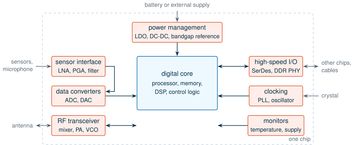
Most of the transistors on a modern chip are digital. They store bits, add numbers and run software, and they are designed by describing behaviour in a hardware language and letting tools place millions of standard gates. Yet almost every useful chip also contains a smaller set of circuits that are designed transistor by transistor, by hand: the analog circuits. They exist because the world outside the chip is not made of bits.
- Sensor interfaces. A microphone, a photodiode or a strain gauge produces a small, continuous voltage or current, often microvolts riding on noise. A low-noise amplifier (LNA), a programmable-gain amplifier (PGA) and a filter must lift it to a level that can be digitized.
- Data converters. An analog-to-digital converter (ADC) turns that voltage into numbers; a digital-to-analog converter (DAC) does the reverse for a speaker, a display or a radio transmitter. The converter’s accuracy is set by analog circuits: comparators, amplifiers and matched capacitors.
- Clocks. Every digital block needs a clean clock. A phase-locked loop (PLL) multiplies a crystal’s few tens of megahertz up to gigahertz, and its timing jitter is an analog noise problem.
- References and power management. A bandgap reference provides a voltage that does not drift with temperature, and low-dropout regulators (LDOs) and DC-DC converters turn a battery’s changing voltage into the clean supplies the rest of the chip needs.
- Input and output. High-speed serial links (SerDes), memory interfaces and radio transceivers are analog circuits that move data off the chip at gigabits per second.
Figure 1.1 places these blocks around a digital core. In a typical mixed-signal system-on-chip the analog part takes only a small fraction of the area, yet it is often the bottleneck in design time and effort [82]. The reason is that analog circuits are judged on continuous quantities: gain, noise, offset, bandwidth, linearity, power. Each depends on the details of the transistors, and no tool can yet synthesize them from a specification.
Every logic gate is an analog circuit
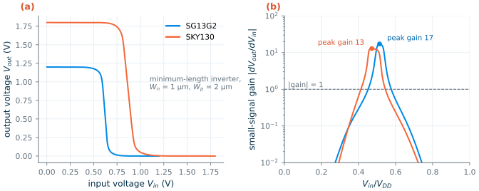
There is a deeper reason why analog never goes away: digital circuits are built from the same transistors, and underneath they behave as analog amplifiers. Figure 1.2 shows the simulated transfer curve of the most basic logic gate, a CMOS inverter made of minimum-length transistors, in each of the two processes this course uses. Far from the switching point the output sits firmly at 0 or at the supply voltage \(V_{DD}\), and a small change at the input does nothing: the gain is far below one. That is what makes digital logic robust. Around the switching point, however, the gate is a high-gain amplifier.
At the point of maximum gain both transistors are in saturation, each behaves as a transconductance \(g_m\) in parallel with an output conductance \(g_{ds}\) (these small-signal quantities are the subject of Chapter 5), and the two drain currents must balance:
\[A_v = \frac{\partial V_{out}}{\partial V_{in}} = -\frac{g_{mn} + g_{mp}}{g_{dsn} + g_{dsp}}. \tag{1.1}\]Worked example 1.1 · The gain of a logic gate
The operating point of each inverter at its point of maximum gain gives, in SG13G2 (\(V_{in}\) = 0.616 V): \(g_{mn}\) = 215 µS, \(g_{mp}\) = 214 µS, \(g_{dsn}\) = 11.8 µS, \(g_{dsp}\) = 13.3 µS. Equation (1.1) gives
\[\vert A_v\vert = \frac{215 + 214}{11.8 + 13.3} = 17.2.\]In SKY130 (\(V_{in}\) = 0.849 V): \(g_{mn}\) = 236 µS, \(g_{mp}\) = 163 µS, \(g_{dsn}\) = 11.8 µS and \(g_{dsp}\) = 19.2 µS, so \(\vert A_v\vert = 399/31.0 = 12.9\).
The slopes of the simulated transfer curves in Figure 1.2 peak at 17.2 and 12.9: the one-line model and the full simulation agree to three digits. The gain exists only because both devices are saturated at once; move the input by about 75 mV in SG13G2 (or 120 mV in SKY130) and one of them leaves saturation and the gain collapses.
The example contains the whole of analog design in miniature: a transistor’s small-signal parameters set the gain, the bias point sets those parameters, and the useful range is limited by the supply. Analog design is the art of keeping transistors in that narrow window on purpose, with feedback, biasing and careful sizing, so that a signal can be amplified without being distorted.
What this means for your design
A lower supply voltage helps digital circuits (less energy per switching event) but hurts analog ones, because the signal has less room. The thermal noise sampled on a capacitor \(C\) has a mean-square value of \(kT/C\) (Chapter 13), so a sine wave that swings over a peak-to-peak range \(V_{pp}\) has a signal-to-noise ratio of
\[\mathrm{SNR} = \frac{V_{pp}^2/8}{kT/C}. \tag{1.2}\]For 80 dB at 27 °C, a signal that could swing over the full supply needs \(C = 8kT\cdot 10^8/V_{pp}^2\) = 2.3 pF at 1.2 V but only 1.0 pF at 1.8 V. The same specification costs about 2.25 times more capacitance, and so area and power, in a 1.2 V process. You will meet this trade-off again and again when the same circuit is designed in SG13G2 and SKY130.
1.2 The analog design flow
Designing an analog block follows a flow with two halves, shown in Figure 1.3. The front end turns a specification into a verified schematic; the back end turns the schematic into polygons that a factory can manufacture.
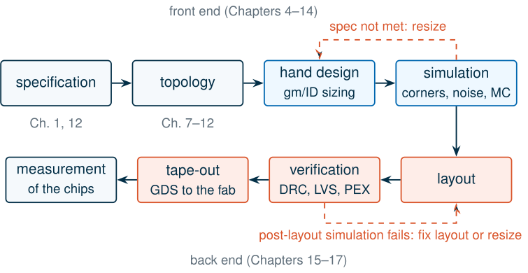
- Specification. Write down what the block must do, with numbers: gain, bandwidth, noise, power, supply, load, temperature range. A specification without numbers cannot be verified.
- Topology. Choose a circuit architecture that can meet it: a single stage or two, a mirror or a cascode. Chapters 7 to 12 build up the menu.
- Hand design. Size every transistor from simple equations and pre-computed device data. This course uses the gm/ID method (Chapter 6), which ties the hand calculation to the PDK’s own models.
- Simulation. Check the design with a circuit simulator (ngspice in this course), first at nominal conditions and then over process corners, temperature, supply and random mismatch (Monte Carlo). Iterate until every specification is met with margin.
- Layout. Draw the transistors, resistors, capacitors and wires as shapes on the layers of the process (Chapter 15). Analog layout is still largely manual, because matching and parasitics depend on geometry.
- Verification. Design-rule checking (DRC) confirms the layout can be manufactured; layout-versus-schematic (LVS) confirms it is the circuit you simulated; parasitic extraction (PEX) adds the resistance and capacitance of the wires, and a post-layout simulation checks that the specification still holds (Chapter 16).
- Tape-out. The finished layout is sent to the foundry as a GDS file, usually on a multi-project wafer (MPW) shared with other designs to split the cost (Chapter 17).
- Measurement. Months later, packaged chips come back and are tested on the bench. Only then do you know whether the models, and your design, were right.
Common pitfall · Treating simulation as the finish line
A schematic that meets every specification at the typical corner is perhaps half finished. Process corners and temperature can move a transistor’s current by 20 % or more (Chapter 3), random mismatch adds offsets of millivolts, and the wires of the layout add capacitance that can halve a bandwidth. Plan for these from the first hand calculation, by designing with margin, rather than discovering them after layout.
1.3 What is in a PDK?
A circuit simulator knows nothing about any particular factory. Everything it needs to know about a manufacturing process comes from the process design kit (PDK), a collection of files that the foundry (the factory) prepares for designers. Figure 1.4 sorts its contents into two groups: what you design with and what your layout is checked against.
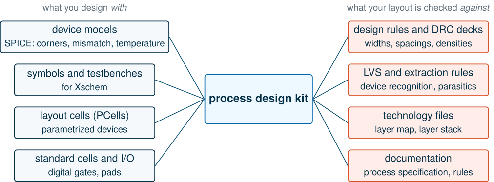
- Device models. SPICE model files for every device the process offers (transistors, resistors, capacitors, diodes, bipolar transistors), fitted to measurements of real wafers. They come in corners that bracket the spread of the manufacturing process, plus statistical versions for Monte Carlo analysis. The models are the single most important part of the PDK for an analog designer: every number in this course comes from them.
- Symbols and testbenches for the schematic editor, so that a transistor placed in Xschem netlists with the right model name and parameters.
- Parametrized layout cells (PCells), which draw a correct transistor, resistor or capacitor from its width, length and number of fingers.
- Standard cells and I/O cells: ready-made logic gates and bond-pad cells for the digital parts of a chip.
- Design rules and DRC decks. Hundreds of rules (minimum widths, spacings, enclosures, densities), in a document and as scripts for the layout tools (Section 3.6).
- LVS and extraction rules, which teach the verification tools how to recognize a device in the layout and how much capacitance a wire has.
- Technology files with the layer map and the layer stack (thicknesses and dielectric constants).
- Documentation: the process specification with measured device parameters, and the layout rules.
In a commercial process, all of this is confidential. You sign a non-disclosure agreement before you see a single model parameter, and you cannot publish your layout, your simulations or often even the process’s name. That is why, until recently, analog IC design was taught with made-up “generic” processes or behind university licence agreements, and why a student project could rarely be shared.
The two PDKs in this course are different: both are published under the Apache 2.0 licence on GitHub, models, rules and all [14, 19]. Inside the IIC-OSIC-TOOLS container they live in /foss/pdks/ihp-sg13g2 and /foss/pdks/sky130A, each with a libs.tech folder (one sub-folder per tool: ngspice, xschem, klayout, magic, netgen, …), a libs.ref folder with the device and cell libraries, and, for IHP, a libs.doc folder with the process specification and layout rules. Chapter 3 opens them up.
1.4 The open-source silicon movement
Three things had to become free before a student could take an analog design from idea to silicon without signing anything: the tools, the PDK and access to a fabrication run. The tools came first. Open-source simulators, schematic editors and layout tools such as ngspice, Xschem, Magic and KLayout have been developed for decades [36, 38, 40, 39]. The missing pieces were the other two, and they arrived in the 2020s. Figure 1.5 shows the main events.
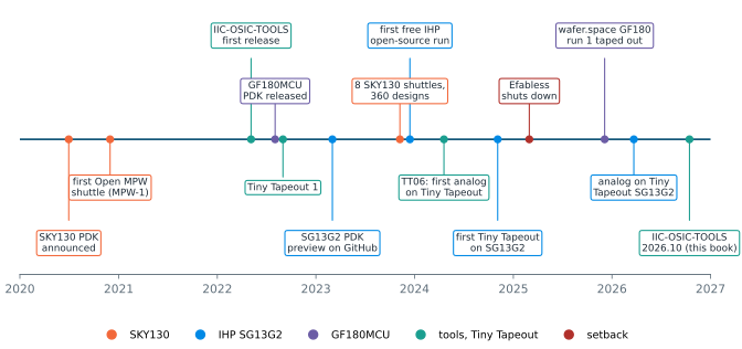
- SKY130 (2020). On 30 June 2020, Google and SkyWater Technology announced the first open-source PDK for a manufacturable process, SkyWater’s 130 nm CMOS technology [21]. Google also paid for free fabrication runs on it, operated by the start-up Efabless, the first of them in November 2020 [21]. Over eight SKY130 shuttles, 360 designs from more than 600 submissions in 19 countries were fabricated free of charge [22]. GlobalFoundries followed with its 180 nm GF180MCU PDK in August 2022 [23].
- The tools in one box (2022). The Department for Integrated Circuits at Johannes Kepler University (JKU) Linz began packaging all the open-source tools and PDKs into a single container image, IIC-OSIC-TOOLS, in 2022 [35]. It is the environment this course uses (Chapter 2).
- Tiny Tapeout (2022). Tiny Tapeout splits one chip on a shuttle into hundreds of small tiles, so that a single design needs only a small fraction of a chip and its cost. Its first run collected designs in August 2022; analog designs were first accepted on TT06 in April 2024 [11, 47].
- IHP SG13G2 (2023). IHP, a German research institute with its own fab, published a preview of its 130 nm SiGe BiCMOS PDK, SG13G2, on GitHub in March 2023, funded by German federal research projects [14]. IHP also ran free open-source shuttles for non-commercial designs from December 2023, with several runs a year in 2024 and 2025; their submissions are public in the Open-Silicon-MPW repository [48].
- A setback (2025). At the start of March 2025 Efabless ceased operations after failing to close a funding round, leaving several shuttles in limbo [24]. Tiny Tapeout survived by moving most of its runs to IHP: its first SG13G2 shuttle closed in November 2024, and since TTIHP26a (March 2026) its SG13G2 runs accept analog designs [12]. SKY130 runs continue through a successor company, and a low-cost GF180MCU service, wafer.space, taped out its first run in December 2025 [12, 26].
SG13G2 vs SKY130 · Getting your design fabricated (November 2026)
For SG13G2, IHP’s free runs have been replaced in 2026 by a low-cost Open-Silicon MPW programme: designs must be released under Apache 2.0 and published on IHP’s GitHub, and the price is a fraction of the normal research rate, with four runs a year [25, 48]. The cheapest route for a small analog block in either process is a Tiny Tapeout tile; check the current shuttle list before you plan a tape-out [12]. Shuttle programmes change from year to year, so treat the details here as a snapshot and Chapter 17 for the submission process.
Open PDKs have changed more than the price. Because the models are public, every number in a paper, thesis or textbook can be reproduced by anyone; designs can be shared, reviewed and reused on GitHub; and courses such as JKU’s [2], IHP’s Analog Academy [3] and this one can show real device data instead of invented values.
1.5 How to use this course
The course has five parts and a set of labs.
Table 1.1. The parts of the course.
| Part | Chapters | What you learn |
|---|---|---|
| I · Getting Started | 1–3 | the flow, the tools and the two PDKs |
| II · The Transistor | 4–6 | how a MOSFET works, its small-signal model, gm/ID sizing |
| III · Building Blocks | 7–10 | amplifier stages, current mirrors, frequency response, the differential pair |
| IV · Amplifiers and Systems | 11–14 | feedback and stability, the two-stage OTA, noise and mismatch, references |
| V · From Schematic to Silicon | 15–17 | layout, verification, fabrication and tape-out |
| Labs | 18 | nine hands-on labs that rebuild the examples in the tools |
Reading paths. Read Parts I and II in order: everything else builds on them. If your goal is a working amplifier quickly, continue with Chapters 7, 8, 10, 11 and 12. If you already know circuit theory and want to get to silicon, read Chapters 3, 6, 12, 15 and 16, then do Labs 6 to 8. If you are an instructor, each chapter matches roughly one week of a semester course, and each lab one afternoon.
Two PDKs, side by side. Every example in the book is worked in both IHP SG13G2 (1.2 V core devices) and SkyWater SKY130 (1.8 V core devices). Netlists and code appear in tabs: choose a PDK once with the tab buttons and every page follows. In plots, SG13G2 is always blue and SKY130 always orange. Comparing the two is one of the most effective ways to learn what in a design depends on the process and what does not.
The boxes. Key equations are framed; worked examples are solved by hand and then checked by simulation; What this means for your design boxes draw the practical lesson; Common pitfall boxes describe mistakes we (or our students) have made; SG13G2 vs SKY130 boxes explain the differences between the processes; Try it boxes point to the matching lab. Long derivations are folded away and can be opened when needed.
Every number is reproducible. Every figure in the course is drawn by a script in the course files from a simulation with the PDKs’ own models, and every process number is cited. If a value in the text surprises you, run the script and check it.
Try it · Lab 0
Before Chapter 2, skim Lab 0: it installs IIC-OSIC-TOOLS and runs the inverter of Figure 1.2 in both PDKs. Change the PMOS width and watch the switching point move.
1.6 The course project
Throughout the course you will design one circuit in depth: a two-stage Miller-compensated operational transconductance amplifier (OTA), the workhorse amplifier of analog design. It is designed in Chapter 12, analysed for noise and mismatch in Chapter 13, laid out in Chapter 15, verified in Chapter 16 and rebuilt in Labs 6 to 8. The specification is the same in both PDKs, at the nominal core supply (1.2 V in SG13G2, 1.8 V in SKY130), the tt corner and 27 °C.
Table 1.2. Specification of the course project, a two-stage Miller OTA.
| Spec | Target |
|---|---|
| Load capacitance | 2 pF |
| Unity-gain bandwidth (GBW) | ≥ 20 MHz |
| Phase margin | ≥ 60° (tt), ≥ 45° over corners |
| DC open-loop gain | ≥ 60 dB |
| Slew rate | ≥ 10 V/µs |
| Output swing | 0.2 V to VDD − 0.2 V |
| Bias | from a 10 µA reference current |
| Power | as low as possible (report it) |
The specification was chosen to be demanding but reachable in both processes, and to expose their differences. Chapter 10 designs a simpler single-stage amplifier, the five-transistor OTA, for the same load and bandwidth, and shows that one stage cannot reach 60 dB of gain, especially in SG13G2, whose short transistors have a much lower intrinsic gain than SKY130’s (Chapter 6). The 1.2 V supply of SG13G2 also leaves less room for the 0.2 V to VDD − 0.2 V output swing: about 0.8 V against 1.4 V in SKY130. Watching how each process forces different design choices for the same specification is the thread that runs through the book.
- Analog circuits connect a chip to the physical world: sensor interfaces, data converters, clocks, references, power management and I/O. They take little area but much of the design effort.
- Even a logic gate is an analog amplifier: a minimum-length inverter has a peak gain of 17 in SG13G2 and 13 in SKY130, and Eq. (1.1) predicts both to three digits.
- The analog flow runs from specification through hand design and simulation to layout, verification, tape-out and measurement, with loops back at every stage.
- A PDK holds everything the tools need to know about a process: models, symbols, layout cells, rules and documentation. Open PDKs publish all of it.
- Since 2020, open PDKs (SKY130, GF180MCU, SG13G2), open tools packaged in IIC-OSIC-TOOLS and low-cost shuttles such as Tiny Tapeout have made it possible to design and fabricate a chip without a licence or a non-disclosure agreement.
- The course project, a two-stage Miller OTA with 20 MHz GBW into 2 pF and 60 dB gain, is designed in both PDKs.
Further reading
- G. Gielen and R. A. Rutenbar [82]: a survey of why analog design resists automation, and what tools can do about it.
- H. Pretl et al., IIC-OSIC-TOOLS [35] and the JKU analog circuit design course [2]: the environment and a complementary course built on the same open tools.
- The Tiny Tapeout analog documentation [47]: what it takes to put your own analog block on a shared chip.
- B. Razavi, Design of Analog CMOS Integrated Circuits [51]: the standard textbook for the circuits in Parts III and IV.