Chapter 2
The Open-Source Analog Toolbox
Xschem, ngspice, KLayout, Magic and Netgen cover the whole analog flow. Packaged together in one container, they install in minutes on Linux, macOS or Windows.
- Name each open-source tool in the analog flow and the job it does.
- Install and start the IIC-OSIC-TOOLS container, pin a release and switch between PDKs.
- Draw a schematic in Xschem, simulate it in ngspice and plot the result.
- Write ngspice control blocks, save device operating points and read results into Python.
Contents
2.1 The tools and what they do
The analog flow of Chapter 1 needs a handful of programs. Figure 2.1 shows which tool does which job, and Table 2.1 lists the versions used throughout this course.
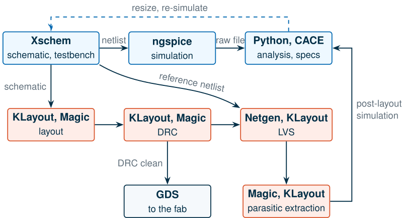
- Xschem is the schematic editor [38]. You place symbols (transistors, sources, the PDK’s devices), wire them, attach simulation commands, and Xschem writes the SPICE netlist: a text file listing every device, its nodes and its parameters. It can also launch the simulator and plot waveforms.
- ngspice is the circuit simulator, the open-source descendant of Berkeley SPICE [36]. It reads a netlist, solves the circuit equations for the analyses you request, and writes the results to a raw file. It accepts compiled Verilog-A models through the OSDI interface [37], which SG13G2 needs.
- KLayout is a layout viewer and editor with a scriptable DRC and LVS engine and a Python interface [39]. Both PDKs ship KLayout DRC and LVS decks.
- Magic is a layout editor with built-in design-rule checking and parasitic extraction [40], the classic tool for SKY130.
- Netgen compares two netlists, one extracted from the layout and one from the schematic, for layout-versus-schematic (LVS) checking [41].
- CACE, the Circuit Automatic Characterization Engine, runs a whole datasheet of simulations (over corners, temperatures and supplies) from one specification file and reports pass or fail [43].
- Python ties everything together: numpy and matplotlib for analysis, and packages such as pygmid [45] and gLayout [44].
Table 2.1. The main tools in IIC-OSIC-TOOLS 2026.10, as reported by the tools themselves.
| Tool | Version | Job | Chapters |
|---|---|---|---|
| Xschem | 3.4.8RC | schematic entry, netlisting, waveform viewing | 2, 7–14, 18 |
| ngspice | 47 | simulation (op, dc, ac, tran, noise, Monte Carlo) | all |
| KLayout | 0.30.12 | layout, DRC, LVS | 15, 16 |
| Magic | 8.3.685 | layout, DRC, parasitic extraction | 15, 16 |
| Netgen | 1.5.324 | LVS | 16 |
| CACE | 2.11.0 | automated characterization | 12, 16 |
2.2 Installing IIC-OSIC-TOOLS
Installing a dozen EDA tools and two PDKs by hand, at compatible versions, takes days. The IIC-OSIC-TOOLS project of the Department for Integrated Circuits at JKU Linz does it once, in a container image that runs the same on Linux, macOS and Windows (on x86 and ARM processors) [35]. A container is a lightweight, isolated Linux environment that runs on top of your operating system through a container engine, Docker or Podman. The image holds about 80 tools and the PDKs for SKY130, GF180MCU, IHP SG13G2 and SG13CMOS5L. Kwantae Kim’s step-by-step guide is a good companion to this section [4].
Install
The project’s interactive installer checks for Git, a container engine (and on macOS the X server XQuartz), offers to install what is missing, asking before each step, and clones the repository with the start scripts [35]. Review it before running it:
# Linux or macOS: download, read, then run the installer
curl -fsSLO https://osic.tools/install.sh && less install.sh && bash install.sh
On Windows, the README gives a PowerShell one-liner. If you prefer to install by hand: install Docker Desktop (macOS, Windows) or Docker Engine (Linux), then clone the repository with git clone --depth=1 https://github.com/iic-jku/iic-osic-tools.git. The image is about 4 GB to download; keep at least 20 GB of disk free [35].
Common pitfall · Fixing Docker permissions the unsafe way
On Linux, “permission denied” on
/var/run/docker.sockmeans your user may not talk to the Docker daemon. Do not run the start scripts withsudoand do not make the socket world-writable (chmod 666): either gives every program on your machine root access. Follow Docker’s post-installation steps for Linux (add your user to thedockergroup, then log out and in), as the IIC-OSIC-TOOLS README instructs, or use rootless Podman, which the start scripts support directly.
Start
The repository contains one start script per way of working; Figure 2.2 shows how each connects your computer to the container.
cd iic-osic-tools
./start_vnc.sh      # full Linux desktop in your browser: http://localhost/?password=abc123
./start_x.sh        # tool windows directly on your desktop through a local X server
./start_shell.sh    # a terminal only (no graphics)
- VNC mode (
start_vnc.sh) runs a complete desktop inside the container and shows it in your web browser through noVNC; nothing else needs to be installed. The default password isabc123; with rootless Podman the port is 8080 instead of 80. It is the easiest mode, and on macOS usually the smoother one for graphics-heavy tools. - X11 mode (
start_x.sh) sends each tool’s window to an X server on your computer: XQuartz on macOS (enable Allow connections from network clients), WSLg on Windows, the desktop’s own server on Linux. Windows then behave like local applications. - Shell mode (
start_shell.sh) is a terminal without graphics, for scripted work such as the figure scripts of this course.
On Windows, use the .bat versions of the scripts.
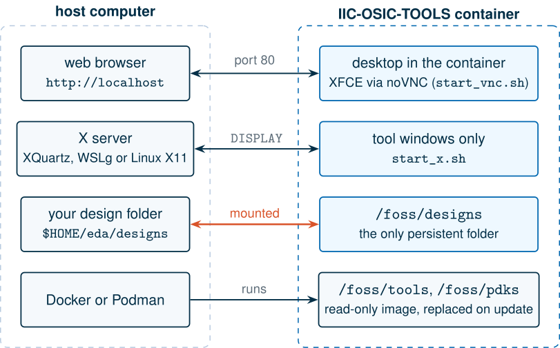
/foss/designs; the tools and PDKs live in the image and are replaced when you update it.Where your files live
The start scripts mount a folder of your computer, by default $HOME/eda/designs (%USERPROFILE%\eda\designs on Windows), into the container as /foss/designs [35]. Save all your work there: everything else inside the container is lost when the container is removed or the image is updated. The tools are in /foss/tools and the PDKs in /foss/pdks (also available as $PDK_ROOT).
Pin a release
By default the scripts pull the latest image. For a course, a thesis or a tape-out, pin the release so that tools and models cannot change under you. This book uses 2026.10:
DOCKER_TAG=2026.10 ./start_vnc.sh
Select a PDK
Inside the container, the variable PDK selects the process for all tools. In release 2026.10 the default is ihp-sg13g2. The command sak-pdk lists the installed PDKs, and switches the current shell to another one by updating PDK, PDKPATH, SPICE_USERINIT_DIR, KLAYOUT_PATH and the standard-cell library:
sak-pdk              # list the installed PDKs
sak-pdk sky130A      # switch this shell to SKY130
sak-pdk ihp-sg13g2   # and back
The switch applies only to the terminal where you typed it, and to the tools you start from it. To make a choice permanent for a design folder, put it in a file called .designinit in /foss/designs, which is sourced every time a shell starts. Because sak-pdk is a shell alias that is not yet defined at that point, call the script behind it:
# /foss/designs/.designinit: start every shell with SKY130 selected
source sak-pdk-script.sh sky130A > /dev/null
We checked this file in the container: a new shell starts with PDK=sky130A and SPICE_USERINIT_DIR=/foss/pdks/sky130A/libs.tech/ngspice.
SG13G2 vs SKY130 · Why the PDK setting matters to the simulator
SPICE_USERINIT_DIRpoints ngspice to the active PDK’s start-up file,.spiceinit. For SG13G2 that file is essential: it loads the compiled PSP transistor model and tells ngspice where the model libraries are (Section 3.5). An SG13G2 netlist simulated from a shell that is switched to SKY130 still works if it names its OSDI files itself, as the scripts of this course do; one that relies on.spiceinitfails with the errors of Section 2.6. Likewise, Xschem picks its symbol libraries fromPDK: open a SKY130 schematic aftersak-pdk sky130A.
2.3 Your first schematic and simulation
Our first circuit is the device testbench of Chapter 6: one NMOS transistor with W = 5 µm and L = 0.5 µm, a gate source and a drain source. The schematics are in the course files under tools/xschem/ch02/ (Lab 0 shows how to download them); copy them into /foss/designs and open the one for your PDK with xschem nmos_tb_sg13g2.sch (or nmos_tb_sky130.sch after sak-pdk sky130A). Figure 2.3 shows them as Xschem draws them.
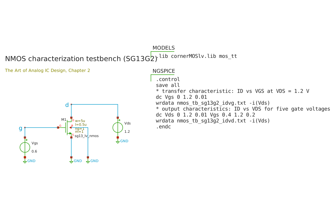
.lib statement, the NGSPICE block the simulation commands.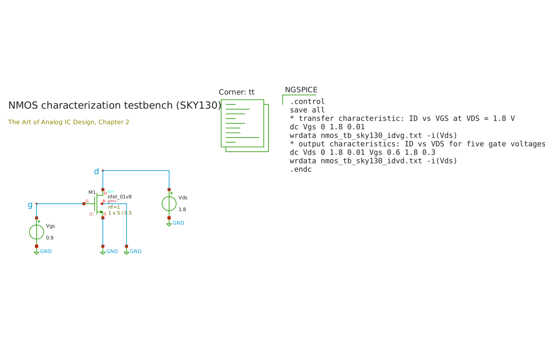
.lib statement, the NGSPICE block the simulation commands.Each schematic has three parts: the circuit (transistor, sources, ground symbols and net labels g and d); a block that loads the PDK’s models; and a block of ngspice commands. In the GUI, the Netlist and Simulate buttons at the top right of the Xschem window write the netlist and run ngspice. The same steps run without a display, which is how we produced the figures:
cd /foss/designs
xschem -n -s -q -x -o simulations nmos_tb_sg13g2.sch   # netlist (-n) in SPICE format (-s), no X (-x), quit (-q)
cd simulations && ngspice -b nmos_tb_sg13g2.spice      # simulate in batch mode
The netlist Xschem writes is short enough to read in full, and you should read it every time something goes wrong:
** sch_path: /foss/designs/nmos_tb_sg13g2.sch
**.subckt nmos_tb_sg13g2
Vgs g GND 0.6
Vds d GND 1.2
XM1 d g GND GND sg13_lv_nmos w=5u l=0.5u ng=1 m=1 mm_ok=1
**** begin user architecture code
.lib cornerMOSlv.lib mos_tt
.control
save all
* transfer characteristic: ID vs VGS at VDS = 1.2 V
dc Vgs 0 1.2 0.01
wrdata nmos_tb_sg13g2_idvg.txt -i(Vds)
* output characteristics: ID vs VDS for five gate voltages
dc Vds 0 1.2 0.01 Vgs 0.4 1.2 0.2
wrdata nmos_tb_sg13g2_idvd.txt -i(Vds)
.endc
**** end user architecture code
**.ends
.GLOBAL GND
.end
** sch_path: /foss/designs/nmos_tb_sky130.sch
**.subckt nmos_tb_sky130
Vgs g GND 0.9
Vds d GND 1.8
XM1 d g GND GND sky130_fd_pr__nfet_01v8 L=0.5 W=5 nf=1 ad=1.45 as=1.45 pd=10.58 ps=10.58 nrd=0.058 nrs=0.058 sa=0 sb=0 sd=0 mult=1
**** begin user architecture code
.lib /foss/pdks/sky130A/libs.tech/combined/sky130.lib.spice tt
.control
save all
* transfer characteristic: ID vs VGS at VDS = 1.8 V
dc Vgs 0 1.8 0.01
wrdata nmos_tb_sky130_idvg.txt -i(Vds)
* output characteristics: ID vs VDS for five gate voltages
dc Vds 0 1.8 0.01 Vgs 0.6 1.8 0.3
wrdata nmos_tb_sky130_idvd.txt -i(Vds)
.endc
**** end user architecture code
**.ends
.GLOBAL GND
.end
A few things are worth noticing. The transistor is an X line, a subcircuit call, because both PDKs wrap their models in subcircuits. The SKY130 corner symbol includes the combined (continuous) model library, whereas the rest of this book uses SKY130’s original binned models (Section 3.5). The SKY130 symbol has filled in the diffusion areas and perimeters (ad, as, pd, ps) from W, assuming 0.29 µm long source and drain regions. The second dc command is a nested sweep: for each value of Vgs it sweeps Vds. The drain current is written as -i(Vds), because ngspice reports the current flowing into a source’s positive terminal. The SG13G2 simulation takes about a second; the SKY130 one about 40 s, almost all of it spent reading the large model library.
Figure 2.4 plots the two files the simulation wrote. These are the familiar MOSFET characteristics of Chapter 4: an exponential, then roughly quadratic, rise of current with gate voltage, and a current that saturates with drain voltage. At full gate and drain voltage the SG13G2 device carries 1.28 mA and the SKY130 device 1.14 mA.
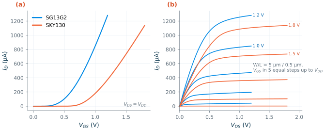
wrdata. (a) ID versus VGS at VDS = VDD. (b) ID versus VDS for five gate voltages up to VDD.2.4 ngspice essentials
An ngspice input file has two parts. The circuit is a list of elements, one per line, whose first letter gives the type: R resistor, C capacitor, V voltage source, X subcircuit, and so on, followed by the nodes and the value. Node 0 (or GND in Xschem netlists) is ground. Lines starting with a dot are dot commands: .lib, .include, .param, .option, .end. The control block, between .control and .endc, is a small script that ngspice runs after reading the circuit: analyses, measurements, printing, plotting and writing files [36].
The listing below simulates a common-source amplifier with a 10 kΩ resistive load and a 1 pF load capacitor, with five analyses. The input bias (0.453 V in SG13G2, 0.883 V in SKY130) was found with a first dc sweep so that the output sits at mid-supply.
* Common-source stage: one netlist, five analyses (SG13G2)
.lib cornerMOSlv.lib mos_tt
VDD vdd 0 1.2
Vin in 0 dc 0.453 ac 1 sin(0.453 10m 1meg)
RD vdd out 10k
CL out 0 1p
XM1 out in 0 0 sg13_lv_nmos W=5u L=0.5u ng=1 m=1
.control
set filetype=ascii
op
print v(out) @n.xm1.nsg13_lv_nmos[ids] @n.xm1.nsg13_lv_nmos[gm] @n.xm1.nsg13_lv_nmos[gds]
write cs_sg13g2.raw
set appendwrite
dc Vin 0 1.2 5m
write cs_sg13g2.raw
ac dec 20 1k 10G
meas ac a0 find vdb(out) at=1k
let a3 = a0 - 3
meas ac f3db when vdb(out)=a3
write cs_sg13g2.raw
tran 2n 3u
meas tran vpp pp v(out) from=1u to=3u
write cs_sg13g2.raw
noise v(out) Vin dec 20 1k 10G
setplot noise1
write cs_sg13g2.raw
.endc
.end
* Common-source stage: one netlist, five analyses (SKY130)
.lib /foss/pdks/sky130A/libs.tech/combined/sky130.lib.spice tt
VDD vdd 0 1.8
Vin in 0 dc 0.883 ac 1 sin(0.883 10m 1meg)
RD vdd out 10k
CL out 0 1p
XM1 out in 0 0 sky130_fd_pr__nfet_01v8 W=5 L=0.5 nf=1
.control
set filetype=ascii
op
print v(out) @m.xm1.msky130_fd_pr__nfet_01v8[id] @m.xm1.msky130_fd_pr__nfet_01v8[gm] @m.xm1.msky130_fd_pr__nfet_01v8[gds]
write cs_sky130.raw
set appendwrite
dc Vin 0 1.8 5m
write cs_sky130.raw
ac dec 20 1k 10G
meas ac a0 find vdb(out) at=1k
let a3 = a0 - 3
meas ac f3db when vdb(out)=a3
write cs_sky130.raw
tran 2n 3u
meas tran vpp pp v(out) from=1u to=3u
write cs_sky130.raw
noise v(out) Vin dec 20 1k 10G
setplot noise1
write cs_sky130.raw
.endc
.end
Run it with ngspice -b cs_sg13g2.cir (batch mode: run, print, exit) or ngspice cs_sg13g2.cir (interactive: run the control block, then wait for commands such as plot v(out)). The analyses are:
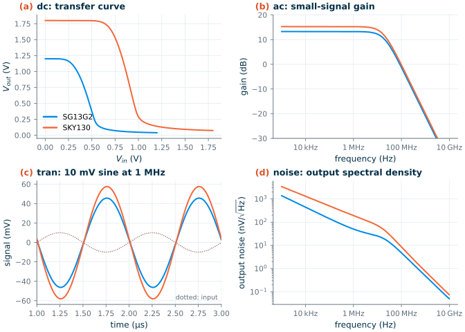
op: the DC operating point, with all capacitors open and inductors shorted. Always run it first and check the node voltages: an amplifier whose output sits at a rail has no gain.dc: the operating point repeated while a source is swept; here the transfer curve \(V_{out}(V_{in})\).ac: a small-signal frequency sweep around the operating point. The source’sac 1sets a 1 V input amplitude, sov(out)is the gain;vdb(out)is the same in decibels.tran: a time-domain simulation with the full nonlinear models; here a 10 mV, 1 MHz sine set by the source’ssin(offset amplitude frequency).noise: the noise spectral density at an output node from every noise source in the circuit, and the equivalent noise at the input.
Device operating points. The @device[parameter] syntax reads internal values of a device, such as its current, \(g_m\) or \(g_{ds}\). The device name is the path through the subcircuits, with a prefix for the device type: n.xm1.nsg13_lv_nmos for SG13G2, because PSP devices loaded through OSDI are N elements, and m.xm1.msky130_fd_pr__nfet_01v8 for SKY130’s built-in BSIM4 M elements. The parameter names differ too: the drain current is ids in PSP and id in BSIM4. To get these values in a sweep, list them in a .save line, as the scripts of Chapter 6 do.
Measurements. meas extracts a number from a result: the value at a point (find ... at=), the point where a signal crosses a level (when), peak-to-peak (pp), averages, rise times. Measurements can use the results of earlier ones through let, as in the −3 dB bandwidth above.
Raw files. write file.raw saves the vectors of the current plot. Each analysis creates a new plot (op1, dc1, ac1, tran1, noise1, …); set appendwrite adds each one to the same file. Raw files are binary by default; set filetype=ascii makes them plain text, which is easy to read from any language. Xschem’s waveform viewer reads either form.
Figure 2.5 shows the four results.
Every simulation result should be checked against a hand calculation. For a common-source stage with a resistive load, the transistor’s output resistance \(r_o = 1/g_{ds}\) appears in parallel with \(R_D\) (Chapter 7), so the low-frequency gain and the bandwidth set by the load capacitor are
\[A_v = -g_m\,(R_D \parallel r_o), \tag{2.1}\] \[f_{-3\,\mathrm{dB}} = \frac{1}{2\pi\,(R_D \parallel r_o)\,C_L}. \tag{2.2}\]Worked example 2.1 · Checking the simulator by hand
The
\[\vert A_v\vert = 558\ \mu\mathrm{S} \times 8.25\ \mathrm{k\Omega} = 4.60 = 13.3\ \mathrm{dB}, \qquad f_{-3\,\mathrm{dB}} = \frac{1}{2\pi \cdot 8.25\ \mathrm{k\Omega} \cdot 1\ \mathrm{pF}} = 19.3\ \mathrm{MHz}.\]opanalysis prints, for SG13G2: \(V_{out}\) = 0.600 V, \(I_D\) = 60.0 µA, \(g_m\) = 558 µS and \(g_{ds}\) = 21.2 µS. Then \(R_D \parallel r_o = 1/(100 + 21.2)\ \mu\mathrm{S}\) = 8.25 kΩ, and Eqs. (2.1) and (2.2) giveThe measurements report
a0= 13.26 dB andf3db= 19.2 MHz, and the transient output swings 91.9 mV peak to peak for a 20 mV input, a gain of 4.59.For SKY130: \(V_{out}\) = 0.909 V, \(I_D\) = 89.1 µA, \(g_m\) = 627 µS, \(g_{ds}\) = 7.34 µS, so \(R_D \parallel r_o\) = 9.32 kΩ, \(\vert A_v\vert\) = 5.85 (15.3 dB) and \(f_{-3\,\mathrm{dB}}\) = 17.1 MHz. Simulated: 15.25 dB (5.79), 17.0 MHz and a transient gain of 5.78.
Hand and simulation agree to about 1 %; the small remaining difference in bandwidth is the transistor’s own drain capacitance, which adds to the 1 pF. Note that the SG13G2 transistor’s \(r_o\) (47 kΩ) loads the 10 kΩ resistor noticeably, the SKY130 one’s (136 kΩ) much less: the lower intrinsic gain of SG13G2 shows up even in this simple stage.
The noise plot in Figure 2.5(d) falls by about √10 per decade of frequency at low frequencies (its power falls tenfold): that is flicker (1/f) noise, which dominates below several megahertz, much more so in SKY130 (192 nV/√Hz at 1 MHz, against 50 nV/√Hz in SG13G2). Above the amplifier’s bandwidth the output noise is filtered by \(C_L\). Chapter 13 explains both.
2.5 Scripting simulations in Python
Clicking through a GUI is fine for one simulation. For a sweep over lengths, corners or PDKs, a script is faster, repeatable and self-documenting. Every figure in this book is drawn by a Python script that writes a netlist, runs ngspice and reads the results; the helper package that does it is part of the course files, under tools/aicd/:
aicd.pdkdescribes both PDKs behind one interface:PDKS["sg13g2"]andPDKS["sky130"]know their supply, minimum length, device names and model libraries.p.mos(...)writes an instance line with the right units for the PDK, andp.op(...)the name of an operating-point value (idsorid,n.orm.).aicd.spice.run(body, pdk, control)adds the model library (and, for SG13G2, the OSDI models), runs ngspice in batch mode, writes every analysis to an ASCII raw file, and returns the results as numpy arrays:res["dc1"]["v(out)"].aicd.lookupreads the gm/ID tables of Chapter 6;aicd.stylesets the colours and sizes of the plots.
The script below sweeps the gate voltage of the testbench of Section 2.3 in both PDKs and prints the current and \(g_m/I_D\) at half the supply. Save it as first_sweep.py at the top of the course files (unpacked into /foss/designs/art_of_aicd) and run python3 first_sweep.py in the container:
"""Sweep VGS of an NMOS in both PDKs and print the current at VGS = VDD/2."""
import sys
sys.path.insert(0, "tools")                 # run from the top of the art_of_aicd repository
from aicd.pdk import PDKS
from aicd.spice import run

for key in ("sg13g2", "sky130"):
    p = PDKS[key]
    body = [f"Vds d 0 {p.vdd}", "Vgs g 0 0",
            p.mos("M1", "n", "d", "g", "0", "0", W=5, L=0.5)]       # W, L in um for both PDKs
    body += p.save_lines("M1", "n", ["id", "gm"])
    dc = run(body, key, [f"dc vgs 0 {p.vdd} 0.01"])["dc1"]
    vgs, ids, gm = dc["v(g)"], dc[p.op("M1", "n", "id")], dc[p.op("M1", "n", "gm")]
    k = abs(vgs - p.vdd / 2).argmin()
    print(f"{p.short}: VGS = {vgs[k]:.2f} V  ID = {ids[k]*1e6:6.1f} uA  gm/ID = {gm[k]/ids[k]:4.1f} 1/V")
SG13G2: VGS = 0.60 V  ID =  196.2 uA  gm/ID =  5.6 1/V
SKY130: VGS = 0.90 V  ID =  106.8 uA  gm/ID =  6.5 1/V
The script took 18 s in the container, most of it for loading the full SKY130 library. Two design choices in the helper are worth copying into your own scripts. First, write lengths once, in micrometres, and let a function add the units, so the scale difference between the PDKs (Section 2.6) cannot bite. Second, read raw files, not printed text: the raw file holds every vector at full precision, and the reader in aicd/spice.py (read_raw, about 40 lines) is short enough to adapt. If you prefer a ready-made package, pygmid and the JKU course’s notebooks use the same approach [45, 2], and CACE automates whole datasheets [43].
Try it · Lab 0
Lab 0 walks through this chapter on your own machine: install IIC-OSIC-TOOLS, pin release 2026.10, open the testbench of Figure 2.3 in Xschem, simulate it from the GUI, then run
first_sweep.py. Finish by switching PDKs withsak-pdkand confirming that both testbenches still run.
2.6 When things go wrong
Simulations fail in a small number of ways, and the error messages are cryptic until you have seen each one. We reproduced the common ones in the 2026.10 container; the messages below are copied from ngspice.
The model library is missing. Forget the .lib line and ngspice does not know what sg13_lv_nmos is:
Error: unknown subckt: xm1 d g 0 0 sg13_lv_nmos w=1u l=0.13u ng=1 m=1
The fix is the .lib statement of Section 3.5. The same message for a SKY130 device means the .lib path is wrong.
The section name is wrong. .lib cornerMOSlv.lib tt instead of mos_tt stops ngspice at once:
ERROR, library file cornerMOSlv.lib, section definition tt not found
SG13G2 sections carry a prefix (mos_tt, res_typ, hbt_typ); SKY130 sections do not (tt).
The SG13G2 start-up file was not read. Running ngspice -n (which skips the start-up files), or from a shell whose SPICE_USERINIT_DIR points elsewhere, produces first
Error: Could not find library file cornerMOSlv.lib
because the model folder is no longer on the search path. Give the full path, .lib /foss/pdks/ihp-sg13g2/libs.tech/ngspice/models/cornerMOSlv.lib mos_tt, and the next error appears:
Unknown model type psp103va - ignored
...
Unable to find definition of model xm1:sg13g2_lv_nmos_psp
ngspice found the model parameters but not the PSP equations, which live in the compiled psp103.osdi. Either restore the PDK environment (sak-pdk ihp-sg13g2) or load the model yourself as the first line of the control block, which is what the scripts of this course do:
.control
pre_osdi /foss/pdks/ihp-sg13g2/libs.tech/ngspice/osdi/psp103.osdi
op
.endc
Common pitfall · Writing W=2u in SKY130, or W=2 in SG13G2
SKY130’s library sets
.option scale=1.0u, soW=2u L=0.15uasks for a 2 pm wide transistor. No model bin covers that, and ngspice stops withcould not find a valid modelnameThe opposite mistake is worse because it is silent. In SG13G2,
W=2 L=0.13means a transistor 2 m wide and 13 cm long. ngspice simulates it without an error and reported a drain current of −128 mA, flowing the wrong way, for a gate voltage of 0.6 V. Always check the operating point of a new circuit: a current that is absurd in size or sign usually means a unit error. Writing sizes through one helper function, asp.mos()does, removes the problem.
A node has no DC path to ground. A node connected only to capacitors (or to transistor gates) has no defined DC voltage. The op analysis then reports
Warning: singular matrix:  check node mid
Warning: True gmin stepping failed
Note: Starting source stepping
Warning: source stepping failed
Note: Transient op started
Note: Transient op finished successfully
and returns a voltage anyway: 0.500 V for a node between two equal capacitors from a 1 V source, the value it would reach if the source were switched on. Add a large resistor (1 GΩ) from the node to ground and op returns 0 V, the true DC solution. Neither answer is “right”; the warning tells you that your circuit does not define the voltage, so fix the circuit, for example with a DC bias path.
Convergence in general. When the Newton iteration of op fails or a transient analysis stops with timestep too small, look first for a modelling error: a floating node, an ideal voltage source in a loop with a capacitor or another source, a switch with zero resistance, a step with zero rise time. Only then reach for simulator options (.option gmin, reltol, method=gear); they can hide problems as easily as they solve them [36].
A last SKY130-specific trap: outside IIC-OSIC-TOOLS, ngspice checks every BSIM4 parameter, and one bin of the SKY130 fs corner fails the check (Fatal: Pclm = -0.00162295 is not positive). The container’s start-up file (~/.spiceinit) sets ng_nomodcheck, which skips the check, and ngbehavior=hsa, without which ngspice picks the SKY130 model bin of a multi-finger transistor from its total width instead of its finger width. Copy both settings into your own .spiceinit if you run the SKY130 models outside the container.
- Xschem draws schematics and writes netlists, ngspice simulates, KLayout and Magic draw and check layouts, Netgen compares netlists, and Python and CACE automate everything.
- IIC-OSIC-TOOLS packages all of them with the PDKs. Start it with
start_vnc.sh(browser) orstart_x.sh(X server), pin the release withDOCKER_TAG, and keep your work in/foss/designs.- The default PDK in 2026.10 is SG13G2;
sak-pdk sky130Aswitches the current shell, and a.designinitfile in/foss/designsmakes a choice permanent.- An ngspice control block runs
op,dc,ac,tranandnoise, extracts numbers withmeas, and writes raw files that Python can read; device values are read with@device[parameter].- Check every simulation by hand: for the common-source stage, \(g_m(R_D\parallel r_o)\) and \(1/(2\pi(R_D\parallel r_o)C_L)\) matched the simulator within about 1 %.
- Most failures are a missing or misnamed
.libsection, OSDI models that were not loaded, a unit-scale mistake betweenW=2andW=2u, or a node without a DC path.
Further reading
- H. Pretl et al., IIC-OSIC-TOOLS README [35], and K. Kim’s installation guide [4]: the authoritative and the friendliest descriptions of the container.
- Ngspice User’s Manual [36]: chapters on analyses, the control language and
measare worth skimming once. - S. Schippers, Xschem manual [38]: symbols, netlisting and the waveform viewer.
- The JKU course’s Xschem and ngspice cheat sheets [2]: one-page references for both tools in SG13G2.