Chapter 9
Frequency Response
Every node has capacitance, so every amplifier has poles. Finding the dominant ones by inspection is the skill that makes compensation and bandwidth design possible.
- Read poles and zeros from a transfer function and sketch Bode plots.
- Apply the Miller approximation and know when it fails.
- Find the poles and the right-half-plane zero of a common-source stage from the gm/ID tables, and check them with ngspice.
- Estimate bandwidth with open-circuit time constants.
- Explain the high-frequency behaviour of followers, common-gate stages and cascodes, and verify it with AC simulation.
Contents
9.1 Poles, zeros and Bode plots
In Chapter 6 we sized a common-source stage so that its gain fell to one at 50 MHz. We treated the load capacitor as the only capacitance in the circuit. It is not. Every node of a real circuit has some capacitance to ground and to its neighbours, and every node is driven through some resistance. A resistance \(R\) charging a capacitance \(C\) cannot follow signals faster than about \(1/(2\pi RC)\), so each node contributes a pole. This chapter is about finding those poles, deciding which of them matter, and checking the answer in both PDKs.
The transfer function
The small-signal behaviour of a linear circuit is described by its transfer function \(H(s) = v_{out}(s)/v_{in}(s)\), a ratio of two polynomials in the complex frequency \(s\). Factored, it reads
\[H(s) = A_0\,\frac{\left(1 + s/\omega_{z1}\right)\cdots}{\left(1 + s/\omega_{p1}\right)\left(1 + s/\omega_{p2}\right)\cdots}, \tag{9.1}\]where \(A_0\) is the low-frequency gain. The roots of the denominator, \(s = -\omega_{p1}, -\omega_{p2}, \dots\), are the poles; the roots of the numerator are the zeros. A pole at \(s = -\omega_p\) lies in the left half of the complex plane and is stable. A zero can lie in either half: we write a left-half-plane (LHP) zero as \((1 + s/\omega_z)\) and a right-half-plane (RHP) zero as \((1 - s/\omega_z)\). We evaluate \(H\) on the imaginary axis, \(s = j\omega = j2\pi f\), to obtain the frequency response.
The simplest case is a single node with resistance \(R\) to AC ground and capacitance \(C\). Its pole is
\[\omega_p = \frac{1}{RC}, \qquad f_p = \frac{1}{2\pi RC}. \tag{9.2}\]This is the whole idea of finding poles “by inspection”: find the resistance and capacitance seen at each node. The rest of the chapter is about the cases where nodes interact, so that Eq. (9.2) needs care.
Bode plots
A Bode plot shows \(\lvert H\rvert\) on a log-log scale and the phase on a log frequency axis. Figure 9.1 shows an example with two poles and a zero. Each factor of Eq. (9.1) changes the slope of the magnitude by 20 dB per decade at its corner frequency, so the magnitude is well described by straight-line asymptotes: −20 dB/dec after the first pole, −40 dB/dec after the second, and the zero bends the curve back by +20 dB/dec. At a pole the exact curve sits 3 dB below the asymptotes, and the phase has moved by 45° of the 90° that the pole eventually contributes.
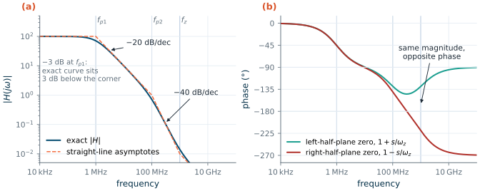
The phase in panel (b) is the reason zeros matter. An LHP zero adds up to +90° of phase and partly undoes a pole. An RHP zero has the same magnitude but subtracts up to 90°, exactly like an extra pole. In a feedback loop this lost phase reduces the phase margin (Chapter 11), which is why we will hunt for RHP zeros in every stage.
The dominant-pole approximation
Multiplying out the denominator of a two-pole transfer function gives
\[1 + b_1 s + b_2 s^2 = \left(1 + \frac{s}{\omega_{p1}}\right)\left(1 + \frac{s}{\omega_{p2}}\right), \quad b_1 = \frac{1}{\omega_{p1}} + \frac{1}{\omega_{p2}}, \quad b_2 = \frac{1}{\omega_{p1}\omega_{p2}}.\]If one pole is much lower than the other, \(\omega_{p1} \ll \omega_{p2}\), the first pole dominates and
Key equation · Dominant-pole approximation
\[\omega_{p1} \approx \frac{1}{b_1}, \qquad \omega_{p2} \approx \frac{b_1}{b_2}. \tag{9.3}\]Valid when the poles are at least a factor of 4 or so apart. Circuit analysis usually gives \(b_1\) and \(b_2\) directly, without factoring.
Equation (9.3) is the workhorse of amplifier analysis [51, 53]: we rarely need the exact roots, only the coefficients of the denominator.
9.2 The Miller effect
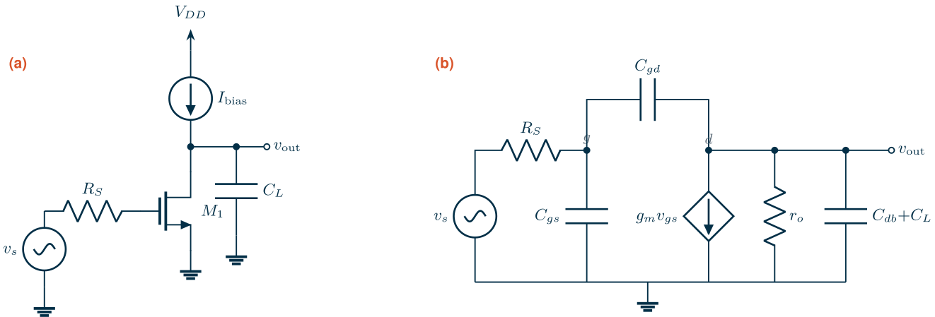
Figure 9.2 shows the circuit we will study throughout this chapter: the common-source (CS) stage of Worked example 6.1, now driven from a source with resistance \(R_S\), and its small-signal model. Three capacitances matter: the gate capacitance \(C_{gs}\) (here all of the gate capacitance except \(C_{gd}\), so \(C_{gs} + C_{gb} = C_{gg} - C_{gd}\)), the gate-drain capacitance \(C_{gd}\), and the capacitance from the output to ground, \(C_{db} + C_L\). The first and last connect a node to ground and fit Eq. (9.2). The middle one connects the input to the output, and that is the problem.
Physical idea
Suppose the stage has a gain of \(-A\) at the frequency of interest. If the gate moves up by 1 mV, the drain moves down by \(A\) mV, so the voltage across \(C_{gd}\) changes by \((1 + A)\) mV. The source must supply \((1 + A)\) times the charge it would supply to the same capacitor connected to ground. Seen from the input, \(C_{gd}\) looks \((1 + A)\) times larger. Seen from the output, the same capacitor changes by \((1 + 1/A)\) times the output swing. This is the Miller effect, first described for vacuum-tube triodes by J. M. Miller in 1920 [81].
Key equation · Miller’s theorem for a capacitor across an inverting gain \(-A\)
\[C_{in} = C_F\,(1 + A), \qquad C_{out} = C_F\left(1 + \frac{1}{A}\right). \tag{9.4}\]For a CS stage, \(C_F = C_{gd}\) and the total input capacitance is \(C_M = C_{gg} + A\,C_{gd}\). If the gain depends on frequency, so does \(C_{in}\): \(C_{in}(\omega) = C_{gg} - C_{gd}\,\mathrm{Re}\{A_v(j\omega)\}\) with \(A_v = -A\) at low frequency.
Hand calculation and simulation
Take the two CS transistors of Worked example 6.1, both carrying 41.9 µA with \(g_m = 628\) µS into \(C_L\) = 2 pF. For this chapter the SG13G2 device is built as four parallel 4.51 µm devices (m=4) instead of two 9.03 µm fingers, so that each matches the 5 µm width of the lookup tables (see the width pitfall in Section 6.6). The tables give:
| Quantity (from the gm/ID tables) | SG13G2, W/L = 18.05/0.75 | SKY130, W/L = 4.62/0.18 |
|---|---|---|
| \(C_{gg}\) | 90.8 fF | 6.44 fF |
| \(C_{gd}\) (intrinsic + overlap) | 10.7 fF | 1.16 fF |
| \(C_{db}\) (intrinsic + junction) | 5.96 fF | 2.11 fF |
| \(r_o = 1/g_{ds}\) | 47.8 kΩ | 68.3 kΩ |
| \(A_0 = g_m r_o\) | 30.1 | 42.9 |
| Miller capacitance \(C_M = C_{gg} + A_0 C_{gd}\) | 411 fF | 56.2 fF |
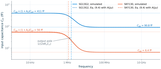
The Miller effect multiplies the SG13G2 input capacitance by 4.5. Figure 9.3 checks the prediction: it plots the input capacitance that ngspice sees, \(C_{in} = \mathrm{Im}\{Y_{in}\}/\omega\), when the gate is driven directly. At low frequency the simulator gives 411 fF and 53.9 fF, within 4 % of the hand values. Above the output pole, at 1.65 MHz and 1.16 MHz, the gain falls, and \(C_{in}\) falls with it, down to \(C_{gg}\) itself.
When the Miller approximation misleads
Equation (9.4) is exact for an ideal amplifier with a fixed gain. A transistor stage is not one: its gain is set by the very capacitances we are trying to model. Three things go wrong when we plug the low-frequency gain into Eq. (9.4) and treat the input and output as two independent poles.
- The gain is not constant. The Miller multiplication collapses above the output pole (Figure 9.3). Using \(A_0\) at high frequencies grossly overestimates the input capacitance.
- It misses the output side. The output node also sees \(C_{gd}\), and through it the source resistance; the poles interact.
- It misses the zero. The feedforward current through the gate-drain capacitance creates an RHP zero (Section 9.3) that a pair of independent poles cannot represent.
Section 9.3 shows by how much the first error can mislead.
9.3 Frequency response of the common-source stage
The exact two-pole result
Writing Kirchhoff’s current law at the gate and the drain of the model in Figure 9.2(b) gives a second-order transfer function. One refinement makes it match the simulator: the charge on the drain responds to the gate voltage through a capacitance \(C_{dg}\) that is not equal to \(C_{gd}\). In a saturated transistor the channel charge is shared between source and drain (in the long-channel limit 60/40), so a change of gate voltage moves channel charge onto the drain while a change of drain voltage hardly moves any charge on the gate. MOSFET capacitances are non-reciprocal [58]. With \(C_o = C_{db} + C_{gd} + C_L\) (all the capacitance on the drain) and \(R_o = 1/g_{ds}\):
Key equation · Common-source stage with source resistance \(R_S\)
\[\frac{v_{out}}{v_s} = -g_m R_o\,\frac{1 - s\,C_{dg}/g_m}{1 + b_1 s + b_2 s^2}, \qquad \begin{aligned} b_1 &= R_S C_{gg} + R_o C_o + g_m R_S R_o C_{gd},\\ b_2 &= R_S R_o\left(C_{gg} C_o - C_{gd} C_{dg}\right).\end{aligned} \tag{9.5}\]The zero is in the right half-plane at \(\omega_z = g_m/C_{dg}\), with \(C_{dg} \approx C_{gdo} + 0.4\,C_{gs,i}\) in saturation (\(C_{gs,i}\) is the intrinsic gate-source capacitance).
Derivation · Eq. (9.5) from the two nodal equations
Let the transistor’s gate charge respond as \(\Delta Q_g = C_{gg}\,v_g - C_{gd}\,v_o\) and its drain charge as \(\Delta Q_d = C_{dd}\,v_o - C_{dg}\,v_g\), where \(C_{dd} = C_{db} + C_{gd}\) is the total drain capacitance with the gate grounded. KCL at the gate and at the drain:
\[\frac{v_s - v_g}{R_S} = s\left(C_{gg} v_g - C_{gd} v_o\right), \qquad g_m v_g + \frac{v_o}{R_o} + s\left(C_{dd}v_o - C_{dg}v_g\right) + sC_L v_o = 0.\]The second gives \(v_o = -v_g\,(g_m - sC_{dg})/(1/R_o + sC_o)\) with \(C_o = C_{dd} + C_L\). Substituting into the first and multiplying by \(R_S R_o\):
\[\frac{v_o}{v_s} = \frac{-g_m R_o\,(1 - sC_{dg}/g_m)}{1 + s\left(R_S C_{gg} + R_o C_o + g_m R_S R_o C_{gd}\right) + s^2 R_S R_o\left(C_{gg}C_o - C_{gd}C_{dg}\right)}.\]With \(C_{dg} = C_{gd}\) and \(C_{gg} = C_{gs} + C_{gd}\) this reduces to the textbook form [51, 53], \(b_1 = R_S[C_{gs} + (1 + g_m R_o)C_{gd}] + R_o(C_{gd} + C_{db} + C_L)\). Notice that \(C_{dg}\) appears only in \(b_2\) and in the zero.
Equation (9.3) applied to Eq. (9.5) is revealing. The coefficient \(b_1\) contains the Miller term \(g_m R_S R_o C_{gd} = R_S \cdot A_0 C_{gd}\), so the dominant pole is slowed by the Miller capacitance seen through \(R_S\) and by the load seen through \(R_o\). The second pole is \(b_1/b_2\): when the load dominates \(b_1\), it is roughly \(1/(R_S C_{gg})\) plus a term set by \(g_m C_{gd}\). At the second pole the input sees \(C_{gg}\), not \(C_M\), exactly as Figure 9.3 showed.
Worked example 9.1 · Poles and zero of the CS stage driven from 20 kΩ
Drive the stages of Worked example 6.1 from \(R_S\) = 20 kΩ, about the output resistance of a gain stage, with \(C_L\) = 2 pF. With the table values above:
SG13G2. \(b_1 = 20\,\mathrm{k}\cdot 90.8\,\mathrm{f} + 47.8\,\mathrm{k}\cdot 2.02\,\mathrm{p} + 628\,\mu\cdot 20\,\mathrm{k}\cdot 47.8\,\mathrm{k}\cdot 10.7\,\mathrm{f} = 1.8 + 96.5 + 6.4 = 104.7\) ns, so \(f_{p1} \approx 1/(2\pi b_1) = 1.52\) MHz. With \(C_{dg} = 10.6 + 0.4\cdot 59.1 = 34.3\) fF, \(b_2 = 1.75\times 10^{-16}\,\mathrm{s^2}\) and \(f_{p2} \approx b_1/(2\pi b_2) = 95.3\) MHz. The exact roots are 1.55 MHz and 93.8 MHz. The zero is at \(g_m/(2\pi C_{dg}) = 2.92\) GHz.
SKY130. \(b_1 = 0.13 + 136.8 + 1.0 = 137.9\) ns: \(f_{p1}\) = 1.15 MHz. \(f_{p2}\) = 1.24 GHz. \(C_{dg} = 2.39\) fF puts the zero at 41.8 GHz.
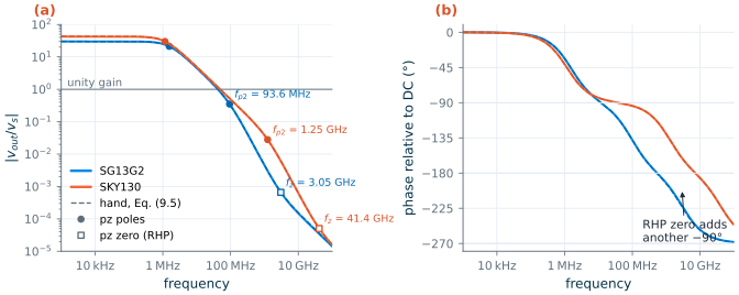
Simulation. ngspice’s pole-zero analysis (Section 9.7) finds the poles at 1.546 MHz and 93.6 MHz (SG13G2) and 1.158 MHz and 1.245 GHz (SKY130), within 1 % of the exact roots, and the RHP zeros at 3.05 GHz and 41.4 GHz, within 5 % and 1 %. Had we used \(C_{gd}\) for the zero we would have predicted 9.37 GHz and 86 GHz, wrong by factors of 3.1 and 2.1.
Figure 9.4 shows the full response. The hand model (dashed) cannot be told apart from the simulation over eight decades. The two PDKs differ in one important way: the SG13G2 transistor needed a 4× longer channel to reach a gain of 30 (Chapter 6), so it has 14× more gate capacitance and its second pole sits at 94 MHz instead of 1.2 GHz. That pole lies just above the unity-gain frequency and pulls it down from the 50 MHz design target to 42.2 MHz, with a phase lag of 113° at that frequency; the SKY130 stage still crosses unity at 49.0 MHz with 91° of lag.
The feedthrough floor of Chapter 6
With \(R_S = 0\), Eq. (9.5) tends to \(C_{dg}/C_o\) at very high frequency: the input couples straight to the output through \(C_{dg}\) and divides against the output capacitance. For the SG13G2 stage this is \(34.3\,\mathrm{fF}/2.02\,\mathrm{pF} = 0.017\), the flattening near 0.015 seen in Figure 6.7. There the coupling was measured as 31 fF of “overlap plus channel charge”: that is \(C_{dg}\), and it is three times \(C_{gd}\).
How badly can Miller mislead?
Now let us do what many designers do in a hurry: treat the input as a separate pole at \(1/(2\pi R_S C_M)\) with the low-frequency Miller capacitance. For the SG13G2 stage with \(R_S\) = 20 kΩ this predicts 19.3 MHz, below the 50 MHz unity-gain target, and we would conclude that the stage cannot work. The true second pole is at 93.6 MHz, almost five times higher. Figure 9.5 repeats the comparison for source resistances from 100 Ω to 1 MΩ.
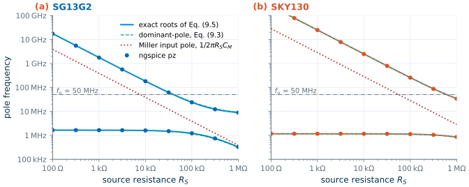
The figure shows three regimes. For small \(R_S\) the output node dominates and the input pole is far away. Only for very large \(R_S\), approaching 1 MΩ in SG13G2, does the input node with its full Miller capacitance become the dominant pole, and only there does the naive estimate approach the truth. In between, where most real stages live, the Miller estimate is low by a factor of 5 (SG13G2) to 9 (SKY130), while the dominant-pole approximation of Eq. (9.3), built from the same capacitances, stays within about 5 % of the simulator everywhere.
Common pitfall · Using the Miller capacitance to place the second pole
\(C_{gg} + A_0 C_{gd}\) is the right capacitance for the input at low frequency and therefore for the dominant pole when the input node is slow. It is the wrong capacitance for any pole above the output pole, because by then the gain that multiplies \(C_{gd}\) has collapsed. Write \(b_1\) and \(b_2\) (or use time constants, Section 9.4) and apply Eq. (9.3) instead.
9.4 Open-circuit time constants
For circuits with more than two capacitors, writing out \(b_1\) by nodal analysis becomes tedious. A shortcut gives \(b_1\) exactly with almost no algebra. It is known as the method of open-circuit time constants (OCTC), or zero-value time constants [53, 9]:
Key equation · Open-circuit time constants
\[b_1 = \sum_k R_{k0}\,C_k, \qquad \omega_{-3\,\mathrm{dB}} \approx \frac{1}{b_1}. \tag{9.6}\]\(R_{k0}\) is the resistance seen by capacitor \(C_k\) with all other capacitors removed (open-circuited) and the input source set to zero.
Each term is a time constant, and the largest one points to the node that limits the bandwidth. Because the estimate uses only \(b_1\), it assumes a dominant pole; when other poles are close it is conservative (it predicts a lower bandwidth than the truth).
For the CS stage the three resistances are easy. \(C_{gs}\) sees \(R_S\). The output capacitance sees \(R_o\). The resistance across \(C_{gd}\) follows from a test current \(i_t\) pushed into one terminal: the gate rises by \(i_t R_S\), which makes the transistor pull \(g_m i_t R_S\) from the drain, so
\[R_{gd,0} = R_S + R_o + g_m R_S R_o.\]The sum \(R_S C_{gs} + R_{gd,0} C_{gd} + R_o (C_{db} + C_L)\) is exactly the \(b_1\) of Eq. (9.5). The Miller effect appears as the large resistance seen by \(C_{gd}\), with no need to talk about multiplied capacitances.
Worked example 9.2 · Bandwidth of a resistively loaded CS stage
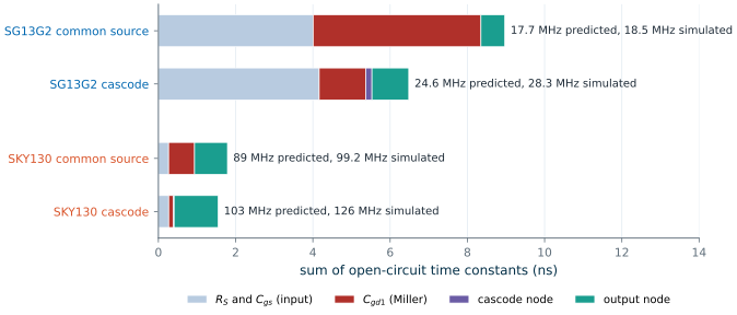
Replace the current-source load by a resistor \(R_D\) that puts the output at \(V_{DD}/2\) (14.3 kΩ in SG13G2, 21.5 kΩ in SKY130), drive the stage from \(R_S\) = 50 kΩ and load it with 50 fF, the input of a following stage. Now \(R_o = R_D \parallel r_o\) = 11.0 kΩ and 16.3 kΩ and the gains are 6.9 and 10.3.
Time constant SG13G2 SKY130 input, \(R_S (C_{gg} - C_{gd})\) 4.01 ns 0.26 ns Miller, \((R_S + R_o + g_m R_S R_o)\,C_{gd}\) 4.35 ns 0.67 ns output, \(R_o (C_{db} + C_L)\) 0.62 ns 0.85 ns sum \(b_1\) → \(f_{-3\,\mathrm{dB}}\) predicted 8.98 ns → 17.7 MHz 1.79 ns → 89 MHz \(f_{-3\,\mathrm{dB}}\) simulated 18.5 MHz 99.2 MHz The estimate is 4 % and 10 % low, on the safe side as expected. In SG13G2 the Miller term is the largest single time constant; in SKY130 the output dominates.
Figure 9.6 shows these sums as bars, together with the cascode stage that we analyse in Section 9.6. The picture says at a glance where the bandwidth goes and therefore what to change.
9.5 Followers and common-gate stages
The source follower
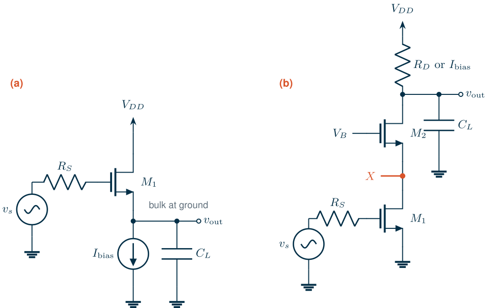
The source follower of Figure 9.7(a) is used as a voltage buffer. Its gain is a little below one, \(g_m/(g_m + g_{mb} + g_{ds})\) (0.877 in SG13G2 and 0.858 in SKY130 for the devices below, with the bulk at ground), and its output resistance is about \(1/(g_m + g_{mb})\). At high frequency it has two energy-storing elements that interact strongly: \(C_{gs}\) connects the input to the output, which follows the input, so the Miller effect works in our favour and \(C_{gs}\) almost disappears from the input. But the follower can ring.
Writing KCL at the gate and the source with \(C_{gs}\), the gate-to-ground capacitance \(C_{gx} = C_{gg} - C_{gs}\), the load \(C_L\) (including the source junction) and \(g_L = g_{mb} + g_{ds}\) gives [51]
Key equation · Source follower driven from \(R_S\)
\[\frac{v_{out}}{v_s} = \frac{g_m + sC_{gs}}{(g_m + g_L) + s\left[C_L + C_{gs} + R_S\left(C_{gx}(g_m + g_L) + C_{gs} g_L\right)\right] + s^2 R_S\left(C_{gs}C_L + C_{gs}C_{gx} + C_{gx}C_L\right)}. \tag{9.7}\]The two poles become complex when \(R_S\) is large, with quality factor \(Q = \sqrt{(g_m + g_L)R_S\Sigma}\,/\,[\ldots]\), where \(\Sigma\) is the bracket multiplying \(s^2 R_S\) and \([\ldots]\) the bracket multiplying \(s\). The response peaks when \(Q > 1/\sqrt{2}\).
The physical reason is visible in the output impedance. With the gate driven through \(R_S\),
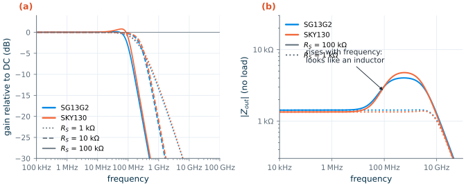
\[Z_{out}(s) \approx \frac{1 + sR_S C_{gs}}{g_m + sC_{gs}},\]which rises from \(1/g_m\) at low frequency towards \(R_S\) at high frequency whenever \(R_S > 1/g_m\). An impedance that rises with frequency behaves like an inductor, and an inductor driving a capacitive load makes a resonant circuit.
How much peaking do real followers show? We sized a follower in each PDK like the CS transistor of Chapter 6 but with L = 0.5 µm (628 µS at 41.9 µA; W = 12.86 µm in SG13G2 and 14.02 µm in SKY130) and loaded it with 0.5 pF. Figure 9.8 gives the answer. With \(R_S\) = 1 kΩ the poles are real (\(Q\) = 0.24) and the bandwidth is about 220 MHz. At 100 kΩ, Eq. (9.7) predicts \(Q\) = 0.74 (SG13G2) and 0.82 (SKY130), and the simulation shows 0.15 dB and 0.8 dB of peaking. The output impedance in panel (b) indeed rises, from 1.4 kΩ to about 4 kΩ, but no further: the gate’s own capacitance to ground, \(C_{gx}\), shunts \(R_S\) at high frequency and caps the rise near \(1/[g_m C_{gx}/(C_{gs} + C_{gx}) + g_L]\), 3.8 kΩ and 4.1 kΩ by hand.
SG13G2 vs SKY130 · How much can a follower ring?
For a large load and ignoring the body effect, Eq. (9.7) reaches its largest quality factor, \(Q_\mathrm{max} \approx \tfrac12\sqrt{C_{gs}/C_{gx}}\), at \(R_S \approx C_L/(g_m C_{gx})\). For the followers here this bound is 0.83 in SG13G2 and 1.12 in SKY130: the SKY130 device has relatively less gate capacitance to ground (\(C_{gs}/C_{gx}\) = 5.1 against 2.8), so it can ring more. The body effect adds the damping conductance \(g_L\) (\(g_m/g_L\) = 6.2 and 4.5 here), which is why neither follower peaks by more than 1 dB. Followers with the bulk tied to the source (a PMOS in its own n-well) lose that damping, and peaking of several dB is common. Always simulate a follower with the actual source impedance and load.
The common-gate stage
In a common-gate stage the signal enters at the source and leaves at the drain, and the gate is at AC ground. No capacitor connects input and output, so there is no Miller effect. The input pole is set by the low resistance looking into the source, about \(1/(g_m + g_{mb})\), and the source capacitance \(C_{gs} + C_{sb}\): this pole lies close to the transit frequency of the device, 1.1 GHz and 15.5 GHz for the CS transistors above. The output pole is set by the output resistance and the load, as in the CS stage. The common-gate stage is therefore fast at its input, which is exactly what makes it a good cascode device.
9.6 Cascode bandwidth
The cascode of Figure 9.7(b) stacks a common-gate transistor \(M_2\) on the common-source transistor \(M_1\). Its well-known benefit is gain (Chapter 7). Its effect on bandwidth depends on the load, and it is worth separating the two cases.
Resistive load: the cascode kills the Miller effect
\(M_1\) now drives the source of \(M_2\), whose resistance is about \(1/g_{m2}\) (1.8 kΩ for our devices, from \(R_x = (r_{o2} + R_D)/(1 + (g_{m2} + g_{mb2}) r_{o2})\)). The gain from the gate of \(M_1\) to the node X is only about \(-g_{m1}/g_{m2} \approx -1\), so \(C_{gd1}\) is multiplied by about 2 instead of \(1 + g_m R_o\). The price is a new pole at X:
\[\omega_x \approx \frac{g_{m2} + g_{mb2}}{C_x}, \qquad C_x = C_{db1} + C_{gs2} + C_{sb2}, \tag{9.8}\]which is close to the transit frequency of \(M_2\): 1.3 GHz in SG13G2 and 13 GHz in SKY130. Back in Figure 9.6, the Miller bar shrinks from 4.35 ns to 1.21 ns in SG13G2 and from 0.67 ns to 0.12 ns in SKY130, while the cascode node adds only 0.16 ns and 0.02 ns. The predicted bandwidth rises from 17.7 to 24.6 MHz and from 89 to 103 MHz; the simulator gives 18.5 → 28.3 MHz and 99 → 126 MHz (Figure 9.9(a)). In SG13G2 the input time constant \(R_S C_{gs}\) of the large transistor now dominates, and only a smaller \(M_1\) or a smaller \(R_S\) would help further.
Capacitive load: same unity-gain frequency, much more gain
With a current-source load and \(C_L\) = 2 pF, the situation of an OTA, the output resistance of the cascode is about \(g_{m2} r_{o2} r_{o1}\) and the dominant pole \(1/(2\pi R_{out} C_L)\) moves down by the same factor that the gain goes up. The unity-gain frequency, \(g_{m1}/(2\pi C_L)\), does not change. Figure 9.9(b) shows it: the gain rises from 30 to 512 in SG13G2 and from 42 to 1019 in SKY130, while the unity-gain frequency stays at 41.5 MHz (was 42.2) and 47.6 MHz (was 49.0).
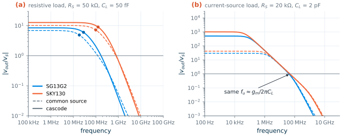
There is a subtlety in panel (b). With the ideal load, the resistance at X is large at DC (the load is a current source), so at low frequency \(C_{gd1}\) is still Miller-multiplied. Only above the output pole, where \(C_L\) shorts the output, does X drop to about \(1/g_{m2}\). With the 20 kΩ source, the SG13G2 cascode’s second pole (76 MHz from pz) is even slightly lower than the CS stage’s (94 MHz), because at those frequencies the CS stage’s own Miller factor has already collapsed to about one while the cascode’s sits at about two.
What this means for your design
Ask what limits the bandwidth before reaching for a fix. If the time-constant bars show a large Miller term, a cascode (or a smaller \(R_S\)) helps. If the load capacitance dominates, as in every OTA driving 2 pF, bandwidth is set by \(g_m/C_L\) alone: a cascode will raise the gain at no cost in speed, and the only way to go faster is more \(g_m\), which means more current or a higher \(g_m/I_D\). The non-dominant poles (the cascode node, the mirror node of Chapter 10) must stay well above \(g_m/(2\pi C_L)\), and the transit frequency of each device tells you whether they will.
9.7 AC analysis in ngspice
An AC analysis linearizes the circuit at its DC operating point and solves it at each frequency. It answers small-signal questions only: it cannot show clipping or slewing, and the AC amplitude of 1 V is a mathematical convenience, not a signal level. Three ngspice commands do almost everything in this chapter [36]:
ac dec 40 1k 100Gsweeps 40 points per decade from 1 kHz to 100 GHz;pz <in+> <in-> <out+> <out-> vol pzcomputes the poles and zeros of the voltage transfer function directly;meas acextracts numbers such as the −3 dB or unity-gain frequency.
The testbench below is the one behind Figure 9.4. The high-gain stage needs its output biased at \(V_{DD}/2\); as in Chapter 6, a very slow DC servo adjusts the gate voltage and is invisible above 1 Hz. The pole-zero analysis is run separately with the gate voltage found by the servo, because the servo’s huge capacitor would add a pole and zero near DC.
* CS stage of Worked example 9.1 (SG13G2): RS = 20k, CL = 2p
.lib cornerMOSlv.lib mos_tt
Vdd vdd 0 1.2
Vin gin 0 dc 0.32 ac 1
Eg  gs gin srv 0 1                  $ gate bias = Vin + servo
Rsrc gs g 20k
XM1 out g 0 0 sg13_lv_nmos W=4.5125u L=0.75u ng=1 m=4
Ib  vdd out 41.89u
CL  out 0 2p
* DC servo: holds v(out) at 0.6 V, open above a few microhertz
Vref ref 0 0.6
Eerr e 0 out ref 1000
Rserv e srv 1e9
Cserv srv 0 1
.control
op
ac dec 40 1k 100G
meas ac f3db when vdb(out)=26.5 fall=1      $ A0 = 29.5 dB
meas ac fu   when vdb(out)=0 fall=1
* for pz: replace the servo by the gate voltage it found, then
* pz gs 0 out 0 vol pz
.endc
.end
* CS stage of Worked example 9.1 (SKY130): RS = 20k, CL = 2p
.lib "$PDK_ROOT/sky130A/libs.tech/ngspice/sky130.lib.spice" tt
Vdd vdd 0 1.8
Vin gin 0 dc 0.775 ac 1
Eg  gs gin srv 0 1                  $ gate bias = Vin + servo
Rsrc gs g 20k
XM1 out g 0 0 sky130_fd_pr__nfet_01v8 W=4.62 L=0.18 nf=1 m=1
Ib  vdd out 41.89u
CL  out 0 2p
* DC servo: holds v(out) at 0.9 V, open above a few microhertz
Vref ref 0 0.9
Eerr e 0 out ref 1000
Rserv e srv 1e9
Cserv srv 0 1
.control
op
ac dec 40 1k 100G
meas ac f3db when vdb(out)=29.5 fall=1      $ A0 = 32.5 dB
meas ac fu   when vdb(out)=0 fall=1
* for pz: replace the servo by the gate voltage it found, then
* pz gs 0 out 0 vol pz
.endc
.end
Common pitfall · Believing every pole that pz prints
The pole-zero analysis works on the complete linearized netlist, including nodes inside the device models. For the SKY130 stage it also reports poles above 800 GHz from the internal body-resistance network of the BSIM4 model, and for SG13G2 a pole and zero at 75 GHz that cancel each other. Discard poles far above the transit frequency and pole-zero pairs that coincide to within a percent. Two practical limits of ngspice-47: run only one
pzper session (a second one in the same.controlblock aborted with an internal error in our runs), and usepzon circuits without huge servo capacitors.
Try it · Lab 3
In Lab 3 you build the common-source amplifier in Xschem. Add a 20 kΩ source resistance, run
acandpzas above, and compare the poles with Eq. (9.5) using your own table values. Then add a cascode device and watch the Miller time constant shrink.
- Every node contributes a pole \(1/(RC)\); the dominant-pole approximation \(\omega_{p1} \approx 1/b_1\), \(\omega_{p2} \approx b_1/b_2\) turns the denominator coefficients into poles without factoring.
- The Miller effect multiplies a gate-drain capacitance by \((1 + A)\), but only while the stage still has gain. Using the low-frequency Miller capacitance for the second pole of a capacitively loaded stage was wrong by about 5× in our SG13G2 example.
- The CS stage has two poles and an RHP zero at \(g_m/C_{dg}\). The drain-gate transcapacitance \(C_{dg}\) (overlap plus about 40 % of the intrinsic \(C_{gs}\)) is two to three times \(C_{gd}\); with it, the hand model matched ngspice to within 5 % in both PDKs.
- Open-circuit time constants give \(b_1\) exactly and show which node limits the bandwidth; the estimate is conservative (4–18 % low here).
- Followers have an inductive output impedance and can peak; with a grounded bulk the body effect kept peaking below 1 dB in both PDKs.
- A cascode buys bandwidth when the load is resistive and gain when it is capacitive; with 2 pF loads the unity-gain frequency stays \(g_m/(2\pi C_L)\).
- SG13G2 needs longer, wider devices for the same gain, so its parasitic poles sit 10× lower than in SKY130: check them early.
Further reading
- B. Razavi, Design of Analog CMOS Integrated Circuits, Chapter 6 [51]: frequency response of all the basic stages, including the Miller effect and follower peaking.
- P. R. Gray, P. J. Hurst, S. H. Lewis and R. G. Meyer [53]: the most complete treatment of zero-value (open-circuit) time constants.
- A. Hajimiri, Analog Circuit Design lectures [9]: a beautiful intuitive development of time-constant methods.
- B. Murmann, Analysis and Design of Elementary MOS Amplifier Stages [7]: an open textbook on single stages, with frequency response.
- Y. Tsividis and C. McAndrew [58]: the transistor capacitance matrix and why \(C_{dg} \neq C_{gd}\).