Chapter 5
Small-Signal Models and Device Characterization
Amplifiers work on small changes around a bias point. The small-signal model captures those changes with a handful of conductances and capacitances, and a simulator can measure every one of them.
- Linearize a MOSFET around its operating point and draw its small-signal model.
- Relate gm, gds and gmb to the bias point and to device size.
- Identify the device capacitances and compute the transit frequency fT.
- Extract small-signal parameters from ngspice for SG13G2 and SKY130 devices, in three independent ways.
- Describe how temperature and process corners move a transistor’s operating point.
Contents
5.1 Linearization
An amplifier’s transistors sit at a fixed operating point (or bias point, or quiescent point Q): DC voltages and currents set by the bias circuit. The signal is a small change on top. If the change is small enough, the transistor’s curved characteristics look straight, and the circuit becomes linear: we can use superposition, impedances, transfer functions and everything else from linear circuit theory.
We write total quantities in upper case with upper-case subscripts (\(I_D\), \(V_{GS}\)), and the small changes in lower case (\(i_d\), \(v_{gs}\)), so that \(V_{GS} = V_{GS,Q} + v_{gs}\). A Taylor expansion of the drain current around Q gives
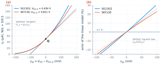
\[I_D(V_{GS,Q} + v_{gs}) = I_{D,Q} + \underbrace{\frac{\partial I_D}{\partial V_{GS}}}_{g_m} v_{gs} + \frac{1}{2}\frac{\partial^2 I_D}{\partial V_{GS}^2}v_{gs}^2 + \dots \tag{5.1}\]The small-signal model keeps only the linear term. How small must \(v_{gs}\) be? Divide the second-order term by the first. For the square law, Eq. (4.5), the ratio is \(v_{gs}/(2V_{OV})\); for the exponential of Eq. (4.9) it is \(v_{gs}/(2nU_T)\). A signal is small when it is much less than twice the overdrive in strong inversion, or than about 60 mV in weak inversion.
Figure 5.1 tests this on the reference device of Worked example 4.1: an NMOS with W/L = 5 µm/0.5 µm, biased at \(I_D\) = 50 µA with \(V_{DS} = V_{DD}/2\). Its overdrive is 0.187 V in SG13G2 and 0.216 V in SKY130, so the square law predicts a 2.7 % and 2.3 % error for a 10 mV signal. The simulated errors are 3.1 % and 2.5 %. At 50 mV they grow to 15 % and 12 %: the linear model is no longer a good description, and the circuit produces distortion.
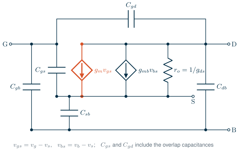
The drain current depends on three voltages, so it has three partial derivatives. Linearizing in all of them gives the small-signal drain current:
\[i_d = g_m v_{gs} + g_{mb} v_{bs} + g_{ds} v_{ds}, \qquad g_m = \frac{\partial I_D}{\partial V_{GS}},\;\; g_{mb} = \frac{\partial I_D}{\partial V_{BS}},\;\; g_{ds} = \frac{\partial I_D}{\partial V_{DS}}. \tag{5.2}\]Each derivative is evaluated at Q, and each depends on Q. Add the capacitances between every pair of terminals and we have the complete model of Figure 5.2, which the rest of this chapter takes apart piece by piece [51, 53, 58].
5.2 Transconductance and output conductance
Transconductance
The transconductance \(g_m\) tells how much drain current a change of gate voltage produces. Differentiating the square law, Eq. (4.5), gives three equivalent forms, and the exponential law of Eq. (4.9) gives a fourth:
Key equation · Transconductance
\[g_m = \mu C_{ox}\frac{W}{L}V_{OV} = \sqrt{2\mu C_{ox}\frac{W}{L}I_D} = \frac{2I_D}{V_{OV}} \quad\text{(strong inversion)}, \qquad g_m = \frac{I_D}{nU_T} \quad\text{(weak inversion)}. \tag{5.3}\]
Which form to use depends on what is held fixed. For a fixed device, \(g_m\) grows with the square root of the current in strong inversion and in proportion to the current in weak inversion. For a fixed current, \(g_m = 2I_D/V_{OV}\) says that a smaller overdrive gives more transconductance, up to the weak-inversion limit \(I_D/(nU_T)\). That trade-off is the subject of the \(g_m/I_D\) method in Chapter 6.
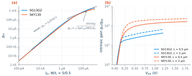
Figure 5.3(a) plots the simulated \(g_m\) against \(I_D\) for the 5/0.5 NMOS on log-log axes, where the two laws are straight lines of slope 1 and ½. Below about 1 µA both devices follow \(I_D/(nU_T)\) closely: at 1 µA the transconductance is 28 µS in SG13G2 and 22 µS in SKY130; the lower slope factor of SG13G2 (Table 4.1) gives it about 25 % more transconductance for the same current. Above about 30 µA they follow the square-root law with the \(\mu C_{ox}\) of Table 4.2. At the highest currents \(g_m\) grows even more slowly, because of velocity saturation and mobility degradation (Section 4.6). The two PDKs give almost the same \(g_m\) for the same current and size, even though their gate voltages differ by 0.4 V.
Output conductance
In saturation the drain current still rises slowly with \(V_{DS}\), through channel-length modulation and DIBL (Section 4.4). The slope is the output conductance \(g_{ds}\), or its inverse, the output resistance \(r_o\). With the Early voltage of Eq. (4.7),
\[g_{ds} = \frac{1}{r_o} \approx \lambda I_D = \frac{I_D}{V_A}. \tag{5.4}\]For a fixed device, \(r_o\) is inversely proportional to the current; for a fixed current, it grows roughly with \(L\), because \(V_A\) does. The reference device has \(g_{ds}\) = 18.9 µS (\(r_o\) = 53 kΩ) in SG13G2 and 4.5 µS (\(r_o\) = 221 kΩ) in SKY130: the same current, a fourfold difference in output resistance, as the Early voltages of Figure 4.5 predict.
Body transconductance
When the bulk voltage changes with respect to the source, the threshold moves (Eq. 4.6), and with it the current. Differentiating gives the body transconductance
\[g_{mb} = \chi\,g_m, \qquad \chi = \frac{\partial V_{TH}}{\partial V_{SB}} = \frac{\gamma}{2\sqrt{2\phi_F + V_{SB}}}. \tag{5.5}\]With the body-effect fits of Table 4.2, \(\chi\) = 0.23/(2√0.85) = 0.125 for the SG13G2 NMOS and 0.41/(2√0.95) = 0.21 for SKY130. The simulator gives \(g_{mb}/g_m\) = 0.127 and 0.210 at the reference bias: the hand estimate is within 2 %. In circuits where the source moves with the signal, such as a source follower, \(g_{mb}\) acts against \(g_m\) and costs gain (Chapter 7).
5.3 Device capacitances and fT
A MOSFET stores charge in three places, and each gives rise to capacitances in Figure 5.2.
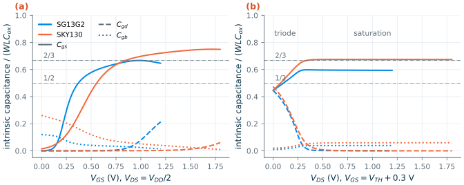
The channel. The inversion charge \(Q_{inv} \approx WLC_{ox}V_{OV}\) belongs to the gate on one side and to the source and drain on the other. How it divides depends on the region. In triode the channel is uniform, so source and drain share it equally: \(C_{gs} = C_{gd} = \tfrac{1}{2}WLC_{ox}\). In saturation the channel is pinched off at the drain end, so the drain no longer affects the charge: integrating the tapered charge of Section 4.3 gives \(C_{gs} = \tfrac{2}{3}WLC_{ox}\) and \(C_{gd} \approx 0\) [58, 51]. Below threshold there is little channel charge, and the gate couples mainly to the bulk through the depletion region, \(C_{gb}\).
The overlap. The gate overlaps the source and drain by a small distance (Figure 4.1), which adds a bias-independent capacitance \(WC_{ov}\) to both \(C_{gs}\) and \(C_{gd}\). From the models, \(C_{ov}\) is 0.64 fF/µm in SG13G2 and 0.25 fF/µm in SKY130.
The junctions. The source and drain diffusions form reverse-biased pn junctions with the bulk, \(C_{sb}\) and \(C_{db}\). They scale with the diffusion area and perimeter (the ad, as, pd, ps parameters in a SKY130 netlist) and shrink as the reverse bias grows. For the 5 µm wide reference device, \(C_{db}\) is 1.6 fF in SG13G2 and 2.3 fF in SKY130.
Putting the first two together, in saturation:
\[C_{gs} \approx \tfrac{2}{3}WLC_{ox} + WC_{ov}, \qquad C_{gd} \approx WC_{ov}, \qquad C_{gg} = C_{gs} + C_{gd} + C_{gb}. \tag{5.6}\]Figure 5.4 shows the intrinsic (channel) parts of the capacitances from the models, normalized to \(WLC_{ox}\), for a long device (W/L = 5/2). In panel (b) the transition from triode to saturation is exactly as described: from 0.45/0.45 (close to ½/½) at \(V_{DS} = 0\) to \(C_{gd} \approx 0\) above about 0.3 V. The saturated \(C_{gs}\) is 0.67 \(WLC_{ox}\) in SKY130 but only 0.60 in SG13G2. Panel (a) shows why the 2/3 rule must be used with care: \(C_{gs}\) rises only gradually through moderate inversion, and in SG13G2 it reaches 2/3 only at the top of the supply range.
The transit frequency
The capacitances set a speed limit. Drive the gate with a small AC current \(i_g\), short the drain to AC ground and measure the drain current \(i_d\). At low frequency the gate draws almost no current, so the current gain \(h_{21} = i_d/i_g\) is huge; as frequency rises, the gate capacitance draws more and more current, \(i_g = j\omega C_{gg}v_{gs}\), while \(i_d = g_m v_{gs}\) stays put. The frequency at which the two are equal is the transit frequency:
Key equation · Transit frequency
\[f_T = \frac{g_m}{2\pi C_{gg}} \;\approx\; \frac{3\,\mu V_{OV}}{4\pi L^2} \quad\text{(long channel, strong inversion)}. \tag{5.7}\]\(C_{gg}\) is the total gate capacitance, overlaps included.
The long-channel form follows from \(g_m = \mu C_{ox}(W/L)V_{OV}\) and \(C_{gg} \approx \tfrac{2}{3}WLC_{ox}\). It says that speed comes from short channels and large overdrive, and that width does not matter: a wider device has more \(g_m\) and more capacitance in the same proportion. For the reference devices, with the effective mobilities of Table 4.2 (286/12.5 = 229 cm²/Vs in SG13G2, 215/7.9 = 271 cm²/Vs in SKY130), Eq. (5.7) gives 4.1 GHz and 5.6 GHz.
Figure 5.5(a) measures \(f_T\) directly, with an AC simulation of \(h_{21}\). The current gain falls at 20 dB per decade and crosses unity at 4.12 GHz in SG13G2 and 5.02 GHz in SKY130. The operating-point values give \(g_m/(2\pi C_{gg})\) = 3.79 and 4.70 GHz, 8 % and 6 % lower, and the long-channel hand estimates are within 8 % and 19 % of these. The small difference between the AC measurement and \(g_m/(2\pi C_{gg})\) comes from the capacitive current that also flows into the drain at high frequency, which is why \(\lvert h_{21}\rvert\) flattens at about 0.4 instead of continuing to fall. Design work, including the lookup tables of Chapter 6, uses \(g_m/(2\pi C_{gg})\).
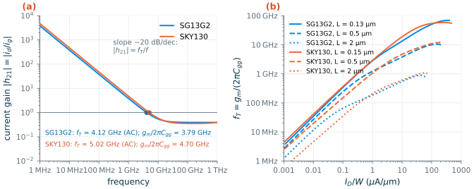
Panel (b) shows \(f_T\) against current density for three lengths. It rises with current density, roughly in proportion in weak inversion and as the square root in strong inversion, and then peaks as velocity saturation and mobility degradation stop \(g_m\) from growing. Minimum-length devices peak at 69 GHz (SG13G2, at 350 µA/µm) and 59 GHz (SKY130, at 260 µA/µm); at L = 2 µm the peak is only about 1 GHz. The \(1/L^2\) dependence of Eq. (5.7) is the strongest lever in analog design.
5.4 Intrinsic gain
Connect an ideal current source to the drain of a transistor and drive its gate: the voltage gain is \(-g_m r_o\). No single-transistor amplifier can do better, so this is called the intrinsic gain:
\[A_0 = g_m r_o = \frac{g_m}{g_{ds}} = \frac{g_m}{I_D}\,V_A = \begin{cases} 2V_A/V_{OV} & \text{strong inversion} \\ V_A/(nU_T) & \text{weak inversion.}\end{cases} \tag{5.8}\]Two levers set it: the inversion level (through \(g_m/I_D\)) and the length (through \(V_A\)). For the reference devices, \(A_0\) is 26 in SG13G2 and 104 in SKY130. Chapter 6 charts \(A_0\) against \(g_m/I_D\) for every length (Figure 6.3); here we look at the third lever, the drain voltage, which matters whenever a stack of transistors must share a small supply.
Figure 5.3(b) plots \(g_m/g_{ds}\) against \(V_{DS}\) at a fixed gate voltage. Below about 0.1 V the device is in triode and the gain is below 6. Just above \(V_{DS,sat}\) it climbs steeply, but full gain needs more drain voltage than the saturation voltage alone: the SKY130 device at L = 0.5 µm has a gain of 31 at 0.2 V, 58 at 0.3 V and 130 at 0.9 V. The SG13G2 device of the same length reaches 17 at 0.2 V, 26 at 0.6 V and 42 at the full 1.2 V.
What this means for your design
Give gain-critical transistors more than their saturation voltage. A rule of thumb of \(V_{DS} \geq V_{DS,sat} + 100\) to 200 mV keeps most of the intrinsic gain; each transistor you stack between the rails eats into that headroom, which is why low-voltage design is hard. In SG13G2 the gain also keeps rising all the way to \(V_{DD}\), so an NMOS that must provide gain should get as much drain voltage as the circuit can spare.
5.5 Extracting parameters with ngspice
Every number in the small-signal model can be measured by simulation. There are three independent ways, and comparing them is the best check that a testbench is right.
- Operating-point values. After an
op(or at every step of adcsweep), ngspice can report each device’s \(g_m\), \(g_{ds}\), capacitances and more, as computed internally by the model. This is fast and gives everything at once, but you must know each model’s parameter names and conventions. - Numerical derivatives of DC sweeps. Sweep \(V_{GS}\) (or \(V_{DS}\), \(V_{BS}\)) in small steps and differentiate the drain current. This uses only terminal currents, so it works for any model, and it is how you would measure a real transistor.
- AC analysis. Put a 1 V AC source on one terminal, and read the small-signal currents: \(g_m = \mathrm{Re}(i_d/v_g)\), \(C_{gg} = \mathrm{Im}(i_g/v_g)/\omega\); move the AC source to the drain for \(g_{ds}\) and \(C_{gd}\), or to the bulk for \(g_{mb}\). This is exactly what the simulator does when it analyses your circuit.
The testbench below does all three for the reference device. Remember that the subcircuit instance XM1 contains the real device, whose path and parameter names differ between the PSP model of SG13G2 and the BSIM4 model of SKY130 (Chapter 3):
* gm and Cgg three ways: SG13G2 NMOS W/L = 5/0.5 at ID = 50 uA, VDS = 0.6 V
.lib cornerMOSlv.lib mos_tt
Vd d 0 dc 0.6
Vg g 0 dc 0.434 ac 1
XM1 d g 0 0 sg13_lv_nmos W=5u L=0.5u ng=1 m=1
.control
* 1. operating-point values (PSP: overlap capacitances are cgsol and cgdol)
op
let gm  = @n.xm1.nsg13_lv_nmos[gm]
let gds = @n.xm1.nsg13_lv_nmos[gds]
let cgg = @n.xm1.nsg13_lv_nmos[cgg] + @n.xm1.nsg13_lv_nmos[cgsol] + @n.xm1.nsg13_lv_nmos[cgdol]
print gm gds cgg                         $ 499.6 uS, 18.92 uS, 20.97 fF
* 2. numerical derivative of a DC sweep (point 10 is VGS = 0.434 V)
dc vg 0.424 0.444 0.001
let gm_num = deriv(-i(vd))
print gm_num[10]                         $ 499.6 uS
* 3. AC analysis at 1 MHz
ac lin 1 1meg 1meg
let gm_ac  = real(-i(vd))
let cgg_ac = imag(-i(vg))/(2*pi*1e6)
print gm_ac cgg_ac                       $ 499.6 uS, 20.97 fF
.endc
.end
* gm and Cgg three ways: SKY130 NMOS W/L = 5/0.5 at ID = 50 uA, VDS = 0.9 V
.lib "$PDK_ROOT/sky130A/libs.tech/ngspice/sky130.lib.spice" tt
Vd d 0 dc 0.9
Vg g 0 dc 0.811 ac 1
XM1 d g 0 0 sky130_fd_pr__nfet_01v8 W=5 L=0.5 nf=1 ad=1.45 as=1.45 pd=10.58 ps=10.58
.control
* 1. operating-point values (BSIM4: overlap capacitances are cgso and cgdo)
op
let gm  = @m.xm1.msky130_fd_pr__nfet_01v8[gm]
let gds = @m.xm1.msky130_fd_pr__nfet_01v8[gds]
let cgg = @m.xm1.msky130_fd_pr__nfet_01v8[cgg] + @m.xm1.msky130_fd_pr__nfet_01v8[cgso] + @m.xm1.msky130_fd_pr__nfet_01v8[cgdo]
print gm gds cgg                         $ 473.6 uS, 4.53 uS, 16.02 fF
* 2. numerical derivative of a DC sweep (point 10 is VGS = 0.811 V)
dc vg 0.801 0.821 0.001
let gm_num = deriv(-i(vd))
print gm_num[10]                         $ 473.6 uS
* 3. AC analysis at 1 MHz
ac lin 1 1meg 1meg
let gm_ac  = real(-i(vd))
let cgg_ac = imag(-i(vg))/(2*pi*1e6)
print gm_ac cgg_ac                       $ 473.6 uS, 16.02 fF
.endc
.end
A note on signs: ngspice reports the current into the positive terminal of a voltage source, so the current flowing into the drain is -i(vd). Table 5.1 lists the operating-point names you will need most often.
Table 5.1. Operating-point parameter names. Prefix each with the device path: @n.xm1.nsg13_lv_nmos[...] (SG13G2) or @m.xm1.msky130_fd_pr__nfet_01v8[...] (SKY130), with your instance name in place of xm1.
| Quantity | SG13G2 (PSP) | SKY130 (BSIM4) |
|---|---|---|
| Drain current | ids |
id |
| \(g_m\), \(g_{ds}\), \(g_{mb}\) | gm, gds, gmb |
gm, gds, gmbs |
| Threshold, saturation voltage | vth, vdss |
vth, vdsat |
| Intrinsic gate capacitance | cgg |
cgg |
| Intrinsic \(C_{gs}\), \(C_{gd}\) | cgs, cgd (positive) |
cgs, cgd (negative: use \(-\)cgs) |
| Overlap capacitances | cgsol, cgdol |
cgso, cgdo |
| Junction capacitances | cjs, cjd |
capbs, capbd |
| Effective W and L | weff, leff |
weff, leff |
Common pitfall · Trusting a parameter name without checking it
The two models do not just use different names; they use different sign conventions. PSP reports the gate-source capacitance as a positive \(-\partial Q_G/\partial V_S\), BSIM4 as the raw derivative \(\partial Q_G/\partial V_S\), which is negative. Both report the overlap capacitances separately from
cgg, so the total gate capacitance iscgg+cgsol+cgdolin SG13G2 andcgg+cgso+cgdoin SKY130. Forget the overlap and the reference device’s \(C_{gg}\) is 30 % too small in SG13G2 and 15 % in SKY130. Before you trust an operating-point value, check it once against an AC simulation, as in Table 5.2.
Figure 5.6 compares the three methods over the whole bias range, and Table 5.2 at the reference bias. They agree to better than 0.05 % for every quantity, in both PDKs. The differences that remain are the step size of the numerical derivative and the 1 MHz frequency of the AC analysis.
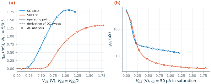
Table 5.2. Small-signal parameters of the reference NMOS (W/L = 5/0.5, ID = 50 µA, VDS = VDD/2), extracted three ways.
| Quantity | SG13G2 op | SG13G2 DC deriv. | SG13G2 AC | SKY130 op | SKY130 DC deriv. | SKY130 AC |
|---|---|---|---|---|---|---|
| \(g_m\) (µS) | 499.5 | 499.5 | 499.6 | 473.2 | 473.2 | 473.1 |
| \(g_{ds}\) (µS) | 18.91 | 18.92 | 18.92 | 4.529 | 4.528 | 4.528 |
| \(g_{mb}\) (µS) | 63.30 | 63.30 | 63.31 | 99.37 | 99.38 | 99.35 |
| \(C_{gg}\) (fF) | 20.97 | 20.97 | 16.02 | 16.02 | ||
| \(C_{gd}\) (fF) | 3.011 | 3.011 | 1.214 | 1.214 |
5.6 Characterizing SG13G2 and SKY130
With the extraction methods in hand, we can describe each process’s core transistors with a few numbers. Table 5.3 is read from the lookup tables of Chapter 6 (built with the operating-point method), at a moderate-inversion bias of \(g_m/I_D\) = 12 V⁻¹ and \(\lvert V_{DS}\rvert = V_{DD}/2\). Everything is per micrometre of width, so it scales to any device made of 5 µm fingers.
Table 5.3. Core devices at gm/ID = 12 V−1, |VDS| = VDD/2, tt, 27 °C (W = 5 µm per finger). VA = (gm/gds)/(gm/ID); Cdd includes the drain junction.
| PDK, device, L | |VGS| (V) | ID/W (µA/µm) | gm/gds | VA (V) | fT (GHz) | Cgg/W (fF/µm) | Cdd/W (fF/µm) | gmb/gm |
|---|---|---|---|---|---|---|---|---|
| SG13G2 NMOS 0.13 µm | 0.536 | 12.9 | 17.6 | 1.5 | 15.9 | 1.55 | 0.33 | 0.11 |
| SG13G2 NMOS 0.5 µm | 0.390 | 6.16 | 26.4 | 2.2 | 2.98 | 3.95 | 0.33 | 0.13 |
| SG13G2 NMOS 2 µm | 0.344 | 1.74 | 40.3 | 3.4 | 0.24 | 14.0 | 0.33 | 0.13 |
| SG13G2 PMOS 0.13 µm | 0.531 | 6.43 | 17.7 | 1.5 | 9.07 | 1.35 | 0.30 | 0.15 |
| SG13G2 PMOS 0.5 µm | 0.492 | 1.67 | 96.7 | 8.1 | 0.75 | 4.23 | 0.30 | 0.19 |
| SG13G2 PMOS 2 µm | 0.478 | 0.44 | 257 | 21.4 | 0.05 | 15.5 | 0.30 | 0.19 |
| SKY130 NMOS 0.15 µm | 0.799 | 18.0 | 20.8 | 1.7 | 27.9 | 1.23 | 0.45 | 0.16 |
| SKY130 NMOS 0.5 µm | 0.759 | 5.77 | 119 | 9.9 | 3.53 | 3.12 | 0.45 | 0.21 |
| SKY130 NMOS 2 µm | 0.713 | 1.65 | 195 | 16.3 | 0.28 | 11.3 | 0.46 | 0.24 |
| SKY130 PMOS 0.15 µm | 0.784 | 2.83 | 8.7 | 0.7 | 5.29 | 1.02 | 0.43 | 0.21 |
| SKY130 PMOS 0.5 µm | 1.087 | 1.34 | 121 | 10.1 | 0.97 | 2.64 | 0.40 | 0.26 |
| SKY130 PMOS 2 µm | 1.146 | 0.34 | 601 | 50.1 | 0.07 | 9.85 | 0.40 | 0.26 |
Read the table by columns. The gate voltages differ by about 0.4 V between the processes, which sets the headroom in every circuit. The current densities are similar for the NMOS devices (the same inversion level needs about the same current per square), while the PMOS devices need 2 to 6 times less current per micrometre, so they must be wider. The NMOS transit frequencies at L ≥ 0.5 µm are within 20 % of each other; only at minimum length does SKY130 pull ahead. The gain column holds the biggest surprise: the SG13G2 NMOS is the weakest device of the four, while the SG13G2 PMOS has about 4 to 6 times more gain than its NMOS partner at 0.5 µm and 2 µm. A designer in SG13G2 should therefore think about putting gain-critical devices in PMOS. The minimum-length SKY130 PMOS, finally, has a gain below 10: avoid it in analog circuits.
Worked example 5.1 · Small-signal model of the reference device by hand
Estimate \(g_m\), \(r_o\), \(C_{gs}\), \(f_T\) and \(A_0\) for the NMOS of Worked example 4.1 (W/L = 5/0.5, \(I_D\) = 50 µA, \(V_{DS} = V_{DD}/2\)), using only the Chapter 4 numbers: \(V_{OV}\) = 0.187 V (SG13G2) and 0.216 V (SKY130), \(V_A\) = 3.4 V and 11.5 V at L = 0.5 µm (Figure 4.5), \(C_{ox}\) = 12.5 and 7.9 fF/µm², \(C_{ov}\) = 0.64 and 0.25 fF/µm.
Transconductance. \(g_m = 2I_D/V_{OV}\) = 100 µA/0.187 V = 535 µS (SG13G2) and 100/0.216 = 464 µS (SKY130).
Output resistance. \(r_o = V_A/I_D\) = 3.4 V/50 µA = 68 kΩ and 11.5/50 µA = 230 kΩ.
Gate-source capacitance. \(C_{gs} = \tfrac{2}{3}WLC_{ox} + WC_{ov}\) = \(\tfrac{2}{3}\cdot 2.5\ \mu\mathrm{m}^2 \cdot 12.5\ \mathrm{fF/\mu m^2} + 5 \cdot 0.64\) fF = 20.8 + 3.2 = 24.0 fF; for SKY130, 13.2 + 1.2 = 14.4 fF.
Transit frequency and gain. \(f_T \approx g_m/(2\pi C_{gs})\) = 3.5 GHz and 5.1 GHz; \(A_0 = g_m r_o\) = 36 and 107.
Quantity SG13G2 hand SG13G2 sim SKY130 hand SKY130 sim \(g_m\) 535 µS 500 µS 464 µS 473 µS \(r_o\) 68 kΩ 53 kΩ 230 kΩ 221 kΩ \(C_{gs}\) 24.0 fF 16.6 fF 14.4 fF 13.8 fF \(f_T\) 3.5 GHz 3.8 GHz 5.1 GHz 4.7 GHz \(A_0\) 36 26 107 104 In SKY130 every estimate is within 10 %. In SG13G2, \(g_m\) is 7 % high, \(r_o\) is 28 % high (the Early voltage of Figure 4.5 was measured at a slightly larger overdrive, and \(V_A\) falls with overdrive in this process) and \(C_{gs}\) is 44 % high: at this moderate-inversion bias the SG13G2 channel capacitance is only 0.43 \(WLC_{ox}\), not 2/3 (Figure 5.4a). The two errors in \(f_T\) partly cancel. The hand model is good for orientation; for numbers you will build on, extract them by simulation.
5.7 Temperature and process corners
A chip must work from cold to hot and on every wafer. Two physical effects make a transistor change with temperature [58, 62]:
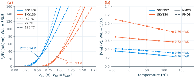
- Mobility falls as the lattice vibrates more, roughly as \(\mu \propto T^{-1.5}\). Less mobility means less current.
- The threshold falls, by roughly 0.5 to 2 mV per kelvin, because the Fermi potential of the substrate shrinks as the temperature rises. A lower threshold means more current.
At small overdrive the threshold wins and the current rises with temperature; at large overdrive the mobility wins and the current falls. In between lies a gate voltage where the two cancel: the zero-temperature-coefficient (ZTC) point.
Figure 5.7 shows both effects. Panel (b) gives the extracted thresholds from −40 °C to 125 °C: the NMOS thresholds fall by 0.76 mV/K (SG13G2) and 0.72 mV/K (SKY130), the PMOS thresholds by 0.61 and 1.76 mV/K. Panel (a) shows the curves crossing at the ZTC point, \(V_{GS}\) = 0.54 V in SG13G2 and 0.93 V in SKY130, both at about 24 µA/µm. The reference device is biased below its ZTC point, so its current at fixed \(V_{GS}\) rises by 23 % (SG13G2) and 20 % (SKY130) at 125 °C and falls by 21 % and 22 % at −40 °C.
Process corners
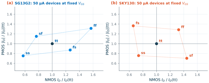
No two wafers are the same: oxide thickness, doping and dimensions vary from run to run. Foundries summarize this variation with corner models that shift the model parameters to the edges of the expected spread (usually ±3σ). tt is typical; ss and ff make both device types slow or fast; the mixed corners make one fast and the other slow. Selecting a corner is a change of one word in the .lib line: mos_ss instead of mos_tt in SG13G2, ss instead of tt in SKY130 (Chapter 3).
Figure 5.8 shows what the corners do. Each NMOS and PMOS of W/L = 5/0.5 is held at the gate voltage that gives 50 µA in tt, and the plot shows the current in each corner relative to tt. In SG13G2 the NMOS current ranges from 0.57× (ss) to 1.57× (ff), and the threshold moves by ±47 mV. In SKY130 the range is 0.74× to 1.32×, and the threshold moves by about ±21 mV in ss/ff, more in the mixed corners. The PMOS spreads are about ±30 % in both.
Common pitfall · Assuming you know which device a corner letter refers to
In SG13G2,
mos_sfmakes the NMOS slow (0.77×) and the PMOS fast (1.15×). In SKY130,sfdoes the opposite: the NMOS is fast (1.44×) and the PMOS slow (0.70×). We checked this with the full SKY130 library in IIC-OSIC-TOOLS. If your design is sensitive to the balance between NMOS and PMOS, as a CMOS inverter’s switching threshold or a class-AB output stage is, simulate both mixed corners, and confirm which is which with a two-transistor test like the one behind Figure 5.8.
What this means for your design
Bias with currents, not voltages. At a fixed gate voltage the corners move the current by up to 60 %, and temperature by another 20 %. If a current mirror (Chapter 8) forces the current instead, the gate voltage absorbs the shift, and \(g_m\), which depends on the current and the inversion level, moves much less. The course OTA (Chapter 12) must keep at least 45° of phase margin over all corners, and you will verify it there.
Try it · Lab 1
In Lab 1 you characterize one NMOS and one PMOS of your PDK: extract \(g_m\), \(g_{ds}\) and \(C_{gg}\) with all three methods of Section 5.5 and confirm that they agree, measure \(f_T\) from \(h_{21}\), and find the ZTC point. Then repeat the corner plot of Figure 5.8 for your own devices.
- Small-signal analysis linearizes the transistor around its bias point. It is accurate to a few per cent for signals well below \(2V_{OV}\) (or about 60 mV in weak inversion).
- \(g_m = 2I_D/V_{OV}\) in strong inversion and \(I_D/(nU_T)\) in weak inversion; \(g_{ds} = I_D/V_A\); \(g_{mb} \approx (0.13\text{–}0.21)\,g_m\) for the reference devices.
- The total gate capacitance includes the overlaps; \(f_T = g_m/(2\pi C_{gg})\) scales as \(1/L^2\) and peaks near 60 to 70 GHz at minimum length in both PDKs.
- Operating-point values, numerical derivatives and AC analysis agree to better than 0.05 % when the testbench is right; check new testbenches this way, and mind the different PSP and BSIM4 names and signs.
- The SG13G2 NMOS has the least intrinsic gain of the four core devices; the SG13G2 PMOS has 4 to 6 times more.
- Thresholds fall by 0.6 to 1.8 mV/K; at fixed \(V_{GS}\) the corners move the current by up to ±60 %, so bias with currents, and remember that
sfmeans opposite things in the two PDKs.
Further reading
- B. Razavi, Design of Analog CMOS Integrated Circuits, Chapter 2 [51]: the small-signal model and its capacitances, derived step by step.
- P. R. Gray, P. J. Hurst, S. H. Lewis and R. G. Meyer [53]: a careful treatment of the MOS small-signal model and its high-frequency limits.
- Y. Tsividis and C. McAndrew [58]: charge partitioning, transcapacitances and the quasi-static approximation in depth.
- The ngspice manual [36]:
op,ac,let,measand device-parameter access with@device[param]. - W. M. C. Sansen, Analog Design Essentials [62]: compact design-oriented notes on transistor models, temperature and corners.