Chapter 27
Matching in Layout
Two devices drawn the same are never the same on silicon. Random variation shrinks with area; systematic variation from gradients, stress and wells only shrinks with layout. This chapter puts numbers on both kinds in SG13G2 and SKY130, models the gradients that layout must cancel, and builds matched resistor, capacitor and transistor arrays from the PDKs' own cells.
- Separate random from systematic mismatch, take the random part from the PDKs’ mismatch models, and estimate both for a layout.
- Model process, thermal and stress gradients and compute what they leave behind in a pair or an array.
- Design common-centroid and interdigitated arrays for resistors, capacitors and transistors, and judge a pattern by the gradient terms it cancels.
- Account for length of diffusion, well proximity and gate density in matched MOS layouts, and know which of these effects each PDK’s models contain.
- Check a matched layout against a short list of rules before verification.
Contents
- 27.1 Random and systematic mismatch
- 27.2 Gradients: process, thermal and stress
- 27.3 Common-centroid and interdigitated arrays
- 27.4 Matching resistors and capacitors
- 27.5 Matching MOS transistors: orientation, LOD, WPE and gate density
- 27.6 Dummies, symmetry and routing
- 27.7 A checklist for matched devices
- Further reading
Chapter 13 extracted the Pelgrom constants of the transistors of both PDKs from their mismatch models and ran Monte Carlo on the offset of an OTA; Chapter 15 laid out the course OTA with an ABBA input pair, a 3 × 3 common-centroid mirror bank and dummies, and showed how strongly the trench next to a gate changes a SKY130 transistor’s current. Chapters 25 and 26 characterized single resistors and capacitors. This chapter is about pairs and arrays: how well two devices can track each other, what makes them drift apart in a predictable way, and what a layout does about it. The resistor and capacitor mismatch comes from Monte Carlo runs of the PDK models, the gradients from a short numerical model, and the layouts from IHP’s KLayout PyCells and Magic’s SKY130 generators, placed and routed by a script [35, 14, 20]:
python3 tools/layout/ch27/match_layouts.py     # PyCells and Magic draw the units; arrays, routing, 3D model
python3 tools/figs/_ch27_sim.py                # Monte Carlo, temperature and LOD runs in both PDKs (about a minute)
python3 tools/figs/ch27_matching.py            # the gradient model, the figures and tools/figs/ch27_numbers.json
27.1 Random and systematic mismatch
Two numbers per pair
Take two devices meant to have the same value \(X\) (a resistance, a capacitance, a drain current) and measure them on one chip. Their relative difference
\[\delta = \frac{X_A - X_B}{(X_A + X_B)/2} \tag{27.1}\]is the mismatch of that pair on that chip. Measured on many chips, \(\delta\) has a mean \(\mu_\delta\) and a standard deviation \(\sigma_\delta\). The mean is the systematic mismatch: every chip has it, with the same sign, because something in the layout or its surroundings treats A and B differently. The standard deviation is the random mismatch: it differs from chip to chip and has no preferred sign [61]. A specification such as “0.1 % at 3σ” needs both, \(\lvert\mu_\delta\rvert + 3\sigma_\delta\), and they call for different cures. Random mismatch falls only with area; systematic mismatch falls with layout, and costs almost nothing once it is understood.
The random part falls with area
The random part comes from microscopic disorder: the number and position of dopant atoms, the grains of a polysilicon film, roughness of the edges, local thickness of a dielectric. Divide a device of area \(a\) into \(N\) small patches of area \(a_0\), each contributing an independent fluctuation of standard deviation \(s\) to the local value. The device’s value is the average over its patches, so its relative spread is \(s/\sqrt{N} = s\sqrt{a_0/a}\), and the difference of two such devices has \(\sqrt 2\) times that. The result is the area law that Pelgrom made famous for transistors [75] and that holds for resistors and capacitors in the same way [111, 61]:
Key equation · Random mismatch of a pair
\[\sigma\!\left(\frac{\Delta R}{R}\right) = \frac{A_R}{\sqrt{WL}} = \frac{A_R}{W}\sqrt{\frac{R_\square}{R}}, \qquad \sigma\!\left(\frac{\Delta C}{C}\right) = \frac{A_C}{\sqrt{A}} = A_C\sqrt{\frac{C_a}{C}}. \tag{27.2}\]\(A_R\) and \(A_C\) (%·µm) are the pair coefficients, \(W\) and \(L\) the resistor’s body, \(A\) the capacitor’s plate area and \(C_a\) its capacitance per area. A resistor of fixed value matches better when it is wider; a capacitor of fixed value can only match better by being larger.
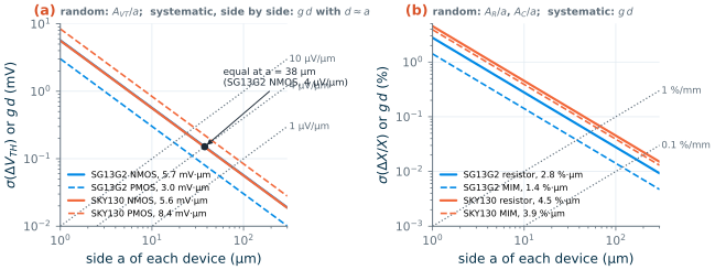
Edges add a second, perimeter term, which matters for narrow resistors and small capacitors. Eq. (27.2) keeps only the area term, which dominates in both PDKs’ models (SG13G2 adds small random width and length terms to its resistors). For transistors, Chapter 13 found \(A_{VT}\) = 5.7 and 3.0 mV·µm for SG13G2’s NMOS and PMOS and 5.6 and 8.4 mV·µm for SKY130’s, by exactly this kind of Monte Carlo experiment.
What the PDK models say about resistors and capacitors
Both PDKs carry local mismatch in their resistor and MIM models, switched on separately from the global corners:
.lib cornerRES.lib res_typ_mismatch     $ rsh 2.0 %um, dW = dL = 6 nm per rppd device
.lib cornerCAP.lib cap_typ_mismatch     $ 1 %um per cmim device
XRa a 0 0 rppd w=2e-6 l=10e-6 b=0 m=1 mm_ok=1
XCa c 0 cap_cmim w=8e-6 l=8e-6 mm_ok=1
.lib "$PDK_ROOT/sky130A/libs.tech/ngspice/sky130.lib.spice" tt_mm   $ mismatch on, no global spread
XRa a 0 0 sky130_fd_pr__res_high_po_1p41 L=10 mult=1 m=1           $ 3.54 %um (body)
XCa c 0 sky130_fd_pr__cap_mim_m3_1 w=8 l=8 mf=1                     $ 2.8 %um
In SG13G2 the instance parameter mm_ok=1 draws the random numbers; the resistor model varies the sheet resistance by 2.0 %·µm per device and the width and length by 6 nm each, and cap_cmim scales its value by 1 %·µm per device [14]. In SKY130 the tt_mm section switches on the MC_MM_SWITCH terms of every model: 3.17, 3.54 and 3.88 %·µm on the bodies of res_high_po_0p69, _1p41 and _2p85, and 2.8 %·µm on cap_mim_m3_1 [19]. These are per-device values; a pair has \(\sqrt 2\) times as much. To check them, _ch27_sim.py places 200 pairs of each size in one netlist, each instance drawing its own random numbers, and reads all 4 000 resistors and 1 600 capacitors from one operating point and one AC point (Figure 27.1).
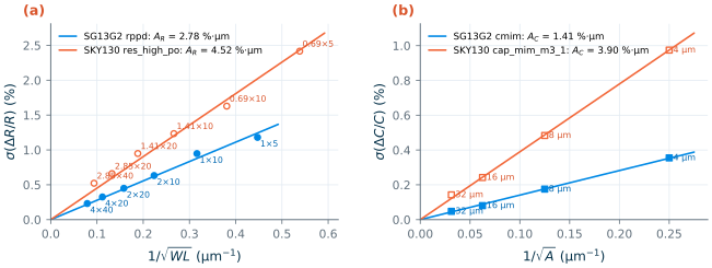
The fits give \(A_R\) = 2.78 %·µm for SG13G2’s rppd (\(\sqrt 2 \times 2.0\) = 2.83 from the model parameter alone) and \(A_C\) = 1.41 %·µm for its cmim (\(\sqrt 2 \times 1.0\)). SKY130’s res_high_po scatters around 4.5 %·µm, a little higher for the wide variant, whose coefficient is larger, and its MIM capacitor reaches 3.90 %·µm (\(\sqrt 2 \times 2.8\)). Table 27.1 collects the coefficients with those of the transistors and turns them into areas.
Table 27.1. Random mismatch of pairs in SG13G2 and SKY130: coefficients from the PDK mismatch models (transistors from Chapter 13, resistors and MIM capacitors from Figure 27.1), and the area each device of a pair needs for σ = 0.1 % (σ = 1 mV for transistors) [14, 19].
| Quantity | SG13G2 | SKY130 |
|---|---|---|
| \(A_{VT}\) NMOS / PMOS | 5.7 / 3.0 mV·µm | 5.6 / 8.4 mV·µm |
| Area per transistor for σ(ΔVTH) = 1 mV, NMOS / PMOS | 32 / 9.2 µm² | 31 / 70 µm² |
| \(A_R\), precision poly resistor | 2.78 %·µm (rppd) |
about 4.5 %·µm (res_high_po) |
| Body area per resistor for σ(ΔR/R) = 0.1 % | 770 µm² | 2 000 µm² |
| \(A_C\), MIM capacitor | 1.41 %·µm (cmim) |
3.90 %·µm (cap_mim_m3_1) |
| Plate area (capacitance) per capacitor for σ(ΔC/C) = 0.1 % | 200 µm² (0.30 pF) | 1 520 µm² (3.0 pF) |
Worked example 27.1 · The random mismatch of a segmented resistor pair, by hand and by Monte Carlo
The resistor arrays of Figure 27.5 build each of two resistors from four series segments:
rppd2 × 10 µm in SG13G2 (1.33 kΩ each, 5.32 kΩ in all) andres_high_po_1p41with L = 10 µm in SKY130 (2.56 kΩ each, 10.24 kΩ). What is σ of the ratio?SG13G2. The four segments are independent, so the resistor behaves like one body of 4 × 2 × 10 = 80 µm². The model parameter gives \(A_R = \sqrt 2 \times 2.0\) = 2.83 %·µm for the sheet resistance, and Eq. (27.2) gives 2.83/√80 = 0.316 %. The heads do not vary in the model and carry 2 × 17.5 Ω of each 1.33 kΩ segment (Chapter 25), so the body is 97.4 % of the resistance: σ = 0.308 %. The Monte Carlo of 200 such pairs gives 0.302 %.
SKY130. Body area 4 × 1.41 × 10 = 56.4 µm², \(A_R = \sqrt 2 \times 3.54\) = 5.01 %·µm, so the body varies by 5.01/√56.4 = 0.667 %; the two heads of 128 Ω each make the body 90 % of each segment: σ = 0.60 %. The Monte Carlo gives 0.66 %, within twice its own sampling uncertainty.
Sizing for σ = 0.1 %. Eq. (27.2) solved for the area: (2.83 × 0.974/0.1)² = 760 µm² per resistor in SG13G2, ten segments of 4 × 20 µm; (5.01 × 0.90/0.1)² = 2 030 µm² in SKY130, 2.7 times as much. In both, segmenting changes nothing about the random part: four segments of 20 µm² match exactly as well as one strip of 80 µm². Segments exist for the systematic part, as the rest of this chapter shows.
The systematic part grows with distance
Suppose a process parameter changes steadily across the die, by a fraction \(g\) per micrometre: a gate-oxide or MIM-dielectric thickness, a doping, a temperature. Two devices whose centres are a distance \(d\) apart then differ by \(g\,d\), whatever their size. Pelgrom’s original paper already wrote the total as two terms [75]:
\[\sigma_{total}^2 \approx \frac{A^2}{\text{area}} + (g\,d)^2. \tag{27.3}\]For two square devices of side \(a\) drawn side by side, \(d \approx a\): the random term falls as \(1/a\) while the systematic term grows as \(a\). Figure 27.2 draws both. With \(A_{VT}\) = 5.7 mV·µm and a gradient of 4 µV/µm, of the order of the distance terms Pelgrom et al. measured, they are equal at \(a = \sqrt{A_{VT}/g}\) = 38 µm; beyond that, making a side-by-side pair larger makes it worse. A common centroid moves \(d\) to zero and removes the second term, which is why large devices and large arrays are the ones that need it most.
The PDKs give no gradient numbers. They are a property of a particular wafer, furnace and package, not of a device model, and they vary from lot to lot. The rest of this chapter therefore treats the gradient as unknown and asks which layouts are insensitive to it.
27.2 Gradients: process, thermal and stress
A gradient model for arrays
Write the relative change of the parameter as a smooth function of position around the centre of an array, and expand it:
\[\varepsilon(x, y) = g_x x + g_y y + \tfrac12\left(h_{xx}x^2 + 2h_{xy}xy + h_{yy}y^2\right) + \dots \tag{27.4}\]A device made of \(n\) units at positions \((x_k, y_k)\), joined in series or in parallel, takes the average of \(\varepsilon\) over its units. The mismatch of devices A and B is the difference of the two averages:
Key equation · Mismatch left by a gradient
\[\delta_{AB} = g_x(\bar x_A - \bar x_B) + g_y(\bar y_A - \bar y_B) + \tfrac12 h_{xx}\left(\overline{x^2}_A - \overline{x^2}_B\right) + h_{xy}\left(\overline{xy}_A - \overline{xy}_B\right) + \tfrac12 h_{yy}\left(\overline{y^2}_A - \overline{y^2}_B\right) \tag{27.5}\]The linear terms vanish when the centroids coincide; the quadratic terms vanish when the devices also have the same second moments about the centre.
Eq. (27.5) is the whole of common-centroid theory. A layout cannot change \(g\) or \(h\); it can only choose the positions. gradient_error() in tools/figs/ch27_matching.py evaluates the left-hand side directly for any field and any placement, which is how the figures of Sections 27.3 and 27.4 were computed.
Process gradients
Furnaces, implanters, deposition and etch tools never treat a whole wafer identically, so oxide and dielectric thicknesses, doping and line widths vary smoothly across it. Over a die the variation looks like a plane plus a little curvature, which is Eq. (27.4) with small coefficients. Wafer-scale gradients are tiny per micrometre: an oxide that is 5 % thinner at the centre of a 200 mm wafer than at its edge changes by only 0.05 %/mm [61]. Local effects near the die edge, near large structures or under dense metal are larger and less regular. Since neither PDK publishes them, design so that the result does not depend on them.
Thermal gradients
A circuit that dissipates power is a heat source, and silicon conducts heat well but not infinitely: about 148 W/(m·K) at room temperature [61]. Near a small source of power \(P\) on the surface of a thick die, heat spreads into a half-space, and the temperature rise at a distance \(r\) and its gradient are
\[\Delta T(r) = \frac{P}{2\pi k\,r}, \qquad \left\vert\frac{dT}{dr}\right\vert = \frac{P}{2\pi k\,r^2}. \tag{27.6}\]For 100 mW, an output stage or a regulator’s pass device, at 200 µm this is 0.54 K and 2.7 K/mm. The bottom of the die and the package cool the far field, so Eq. (27.6) overestimates at distances comparable with the die thickness, but it shows the shape: a field that is curved everywhere and steepest near the source. What it does to a matched pair depends on how the parameter moves with temperature. At 5 µA, the gate-source voltage of a 4/1 µm transistor moves by −0.53 mV/K (SG13G2 NMOS), −0.34 mV/K (SG13G2 PMOS), −0.49 mV/K (SKY130 NMOS) and −1.34 mV/K (SKY130 PMOS) in the PDK models; the precision resistors move by 140 ppm/K (rppd) and 474 ppm/K (res_high_po) (Chapter 25); the SG13G2 MIM capacitor by 3.6 ppm/K (Chapter 26).
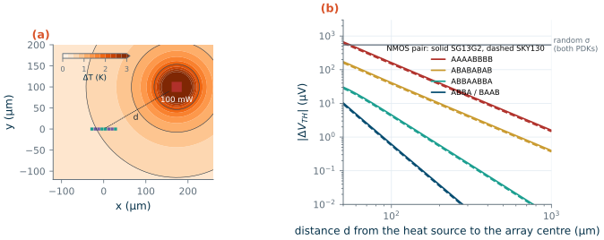
Figure 27.3 evaluates Eq. (27.5) in the field of Eq. (27.6) for an NMOS pair. Side by side (AAAABBBB) the pair sees a temperature difference of 0.075 K at 200 µm, 40 µV of offset in SG13G2; interleaved (ABABABAB) a quarter of that; as the common-centroid row ABBAABBA 0.6 µV; as the two-row ABBA/BAAB 0.04 µV. The random σ of the same pair is 540 µV. Two conclusions follow. Thermal gradients from a block’s own bias currents are harmless; they matter near output stages, regulators and heaters, and for precision references and converters. And a common centroid cancels them so thoroughly that a distance of a few hundred micrometres plus a good pattern makes them disappear. Place matched devices on an axis of symmetry of the heat sources, so that the remaining curvature is symmetric about the array too [61].
Stress gradients
The third gradient is mechanical. Mould compound, die attach and lead frame expand with temperature more than silicon does, so a packaged die is under stress that is largest near its edges and corners and most uniform near its centre. Silicon is piezoresistive: its resistivity and carrier mobility change under stress, by different amounts for electrons and holes and for different crystal directions. Polysilicon, made of randomly oriented grains, is far less sensitive than monocrystalline silicon, which is one reason why the precision resistors of both PDKs are poly; MIM capacitors are nearly immune, because the change of plate area and of permittivity partly cancel [61]. Neither PDK models package stress, so the guidance is qualitative: keep critical matched devices away from the die edges and corners, preferably near the centre or on one of the die’s axes of symmetry, and lay them out as common centroids so that the remaining stress gradient cancels. The stress that the shallow trench puts on a transistor next to it is a local effect, and SKY130 does model it (Section 27.5).
27.3 Common-centroid and interdigitated arrays
What a pattern cancels
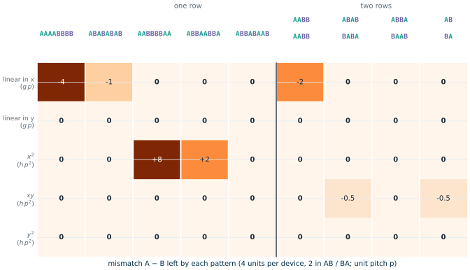
Chapter 15 compared four one-row arrangements under a parabola. Eq. (27.5) lets us grade any arrangement in two dimensions, term by term. Figure 27.4 does so for nine patterns of two devices with four units each (two in the smallest): the entries are the five coefficients of Eq. (27.5), in units of \(g\,p\) and \(h\,p^2\) for a unit pitch \(p\).
Reading the table:
- Side by side (AAAABBBB) leaves the full linear term, four pitches’ worth. Interleaving (ABABABAB) reduces it to one pitch but does not cancel it, because the A units always sit half a pitch to the left of their B neighbours.
- Any symmetric arrangement (AABBBBAA, ABBAABBA, ABBABAAB) cancels both linear terms: the centroids coincide. Hastings calls this the rule of coincidence, and adds symmetry about both axes as the second rule [61].
- Curvature separates the good from the best. AABBBBAA puts A at both ends and B in the middle, so their second moments differ by 8 \(h p^2\); ABBAABBA, two small common centroids side by side, leaves 2; ABBABAAB leaves nothing, because A and B also share their spread about the centre. This is the rule of dispersion: an array built from several small common-centroid groups is better than one large group, because the quadratic residue of each group scales with the square of its own span [61]. The fourth rule, compactness, follows from the same square: keep each group as short as possible.
- Two dimensions. The cross-coupled quad AB/BA, the classic arrangement for a pair of capacitors or transistors, cancels the linear terms and the \(x^2\) and \(y^2\) curvature, but leaves \(-\tfrac12 h_{xy}p^2\) of the saddle term, as does the checkerboard ABAB/BABA. ABBA/BAAB cancels all five terms. It is the two-dimensional version of ABBABAAB and the arrangement to prefer when a pair has four or more units per device.
Real fields are not polynomials, but Eq. (27.4) is their Taylor expansion, so a pattern that cancels the first and second orders leaves only the third, which shrinks as the cube of the array’s size relative to the scale of the field. That is why the ABBA/BAAB curve of Figure 27.3b falls so much faster than the others.
Ratios and many devices
The rules extend to unequal devices. A ratio of 1 : 4 drawn as AABAA, or 1 : 2 : 4 in a symmetric two-dimensional pattern, keeps every centroid at the centre; a single unit, which cannot be split, goes in the middle. For arbitrary ratios one either accepts an approximate centroid, scattering the units as evenly as possible, or builds the ratio from series–parallel combinations of identical units [61]. The binary-weighted capacitor array of Section 27.4 is an example with five devices in sixteen units.
What this means for your design
Grade a placement by Eq. (27.5), not by eye. For a pair with two units each, use ABBA (one row) or AB/BA (a quad); with four or more each, ABBABAAB or ABBA/BAAB, which cancel curvature too; for large arrays, tile small common-centroid groups instead of drawing one big symmetric pattern. The arrangement costs no area, only routing, so there is no reason ever to place a matched pair side by side, even where Figure 27.2 says the gradient term would be small today.
27.4 Matching resistors and capacitors
A matched resistor array
Figure 27.5 shows the pair of Worked example 27.1 as drawn by match_layouts.py. The segments are unmodified copies of one PDK generator cell: IHP’s rppd PyCell (2 × 10 µm) and Magic’s res_high_po_1p41 (L = 10 µm), at a pitch of 3.0 and 1.89 µm. The pattern is D ABBAABBA D: two small common-centroid groups side by side (dispersion), with a dummy segment at each end. Its construction follows the rules every precision resistor array uses [61]:
- Identical, straight segments of the same width and orientation. A wider resistor is made of segments in parallel, never of one wider strip, so that width bias and edge roughness scale the same way in both devices (Chapter 25). Straight segments joined in metal have no turns, whose corners are where the film is least controlled.
- Heads in series in equal numbers. Each resistor here has four segments and so eight heads; the head resistance, which varies differently from the body, enters both resistors equally.
- Current flowing both ways. Each resistor has two segments carrying current upwards and two downwards. Effects that depend on the direction of current or of the heads (a misaligned contact, a small thermoelectric voltage between heads at different temperatures) cancel within each resistor.
- Jumpers outside the bodies. The series connections leave each head on a stub one metal up (Metal2, met2) and run on tracks two metals up (Metal3, met3) beyond the heads, “folded out”, so that no wire crosses a resistor body. Where a wire must cross, it should cross every segment the same way.
- Dummies with the same pitch and shape, tied to a quiet node. The end segments would otherwise see an open field on one side and etch, implant and fill differently from the inner ones. Here both heads of each dummy go to a ring on the track layer, which is connected to ground or to the substrate tie.
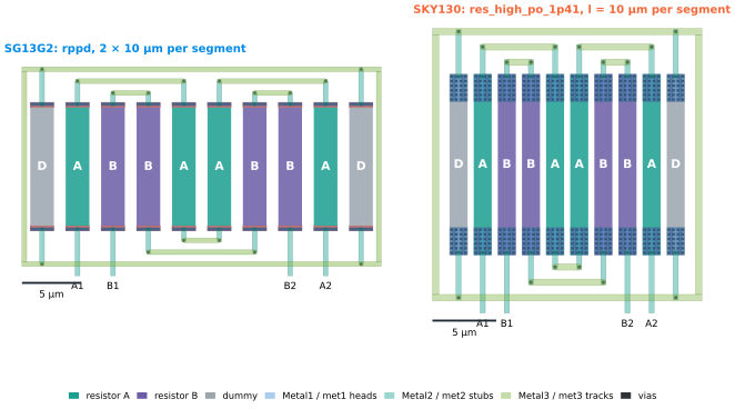
rppd, 2 × 10 µm, 5.32 kΩ per resistor, array 30.4 × 17.7 µm. SKY130: Magic's res_high_po_1p41, L = 10 µm, 10.2 kΩ per resistor, array 21.1 × 22.3 µm. Generated by tools/layout/ch27/match_layouts.py; layer colours as in the 3D gallery.The SKY130 array is the narrower one although each segment has twice the resistance, because res_high_po is a narrower, higher-sheet film; it is also the taller one, because Magic’s heads are 2.1 µm long against 0.43 µm for the PyCell. The random part of both arrays is in Worked example 27.1. Their systematic part, by Figure 27.4, is \(2h p^2\) of curvature along the row and nothing else. Both arrays, and both capacitor arrays of Figure 27.6, pass the PDKs’ KLayout rule decks (match_layouts.py drc, without the chip-level density checks).
A matched capacitor array
Capacitor arrays follow the same logic with a few rules of their own [111, 61]. Every capacitor is a whole number of identical unit capacitors, so that the perimeter term of Eq. (26.2) and the etch bias of the plate edges scale with the ratio exactly; a ratio of 1 : 2.5 is better drawn as 2 : 5 units than with a larger unit. A ring of dummy units gives every active unit the same neighbours. The top plate, which faces nothing but the bottom plate (Chapter 26), goes to the sensitive node, the comparator or amplifier input of a switched-capacitor circuit, and the bottom plates to the switches. And the wiring must give every unit the same parasitic: a stub from each unit to a track is a small capacitor of its own, and if one capacitor’s units have longer stubs than another’s, the ratio moves by the difference.
Figure 27.6 applies this to a binary-weighted array of 1 : 1 : 2 : 4 : 8 units, the capacitive DAC of a 4-bit successive-approximation converter (Chapter 21) [110]. The 16 units of 5 × 5 µm (about 38 fF in SG13G2 and 53 fF in SKY130) form a 4 × 4 core inside a ring of 20 dummies whose two plates are shorted together. C4 takes one colour of a checkerboard; C3 four units on a tilted rectangle around the centre; C2 two opposite corners; C1 and C0, single units that cannot have a centroid at the centre, sit next to it. Every capacitor with two or more units therefore has its centroid at the centre of the array. The top plates are joined by a mesh one metal above the unit’s own top contact (TopMetal1 in SG13G2, met5 in SKY130) and leave the array on TopMetal2 or met5; each bottom plate drops through one via to a stub under its own plate, which shields the stub from the top plate, and into a channel below its row, where one track per capacitor collects the units of that row and runs to one spine per capacitor on the left. Where the top-plate mesh bridges a channel it crosses the tracks below it, and every crossing adds a small capacitance between the top plate and that track’s capacitor. Here the crossings are not equal per unit; a production array gives every capacitor the same number of crossings per unit, or puts a grounded shield plate between the tracks and the mesh, and checks the result in an extraction.
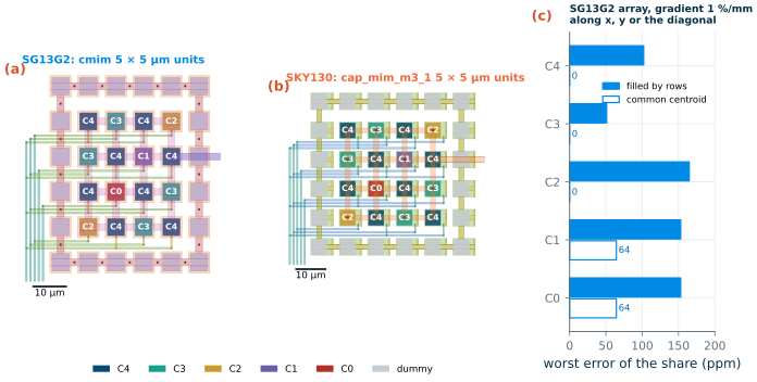
cmim (56 × 60 µm) and SKY130 cap_mim_m3_1 (63 × 55 µm), drawn by the PDK generators and routed by match_layouts.py. (c) Error of each capacitor's share of the total under a linear gradient of 1 %/mm along x, y or the diagonal (worst of the three), for the unit positions of the SG13G2 layout, filled row by row (C4 in the top two rows) and in the common-centroid assignment shown; the SKY130 layout gives values within 10 %.Worked example 27.2 · Random against systematic in the capacitor array, by hand and from the layout
Random part. One 5 × 5 µm unit varies by \(A_C/(\sqrt 2 \cdot 5\ \mu\text{m})\): 1.41/7.07 = 0.20 % in SG13G2 and 3.90/7.07 = 0.55 % in SKY130. The largest step of the DAC, at mid-scale, switches C4 in and C0 to C3 out; its error in units of the LSB is \((C_4 - C_0 - C_1 - C_2 - C_3)/C_u\), a sum of 16 independent unit errors: σ = 4 × 0.20 % = 0.008 LSB (SG13G2) and 0.022 LSB (SKY130).
Systematic part, filled by rows. If C4 fills the top two rows, its centroid lies one row pitch \(p_y\) above the centre of the core, and C0 to C3 (the lower two rows) one pitch below. A gradient \(g\) along y then makes C4 larger by \(g p_y\) and the rest smaller by the same amount, so the mid-scale step is off by \(8 \cdot 2 g p_y\) = \(16 g p_y\) units. With the layout’s row pitch of 10.2 µm (SG13G2) and g = 1 %/mm = 10⁻⁵/µm, C4’s share is off by \(g p_y\) = 102 ppm and the step by 0.0016 LSB; the script, evaluating Eq. (27.5) on the unit positions of the generated layout, gives the same 102 ppm (Figure 27.6c), and 94 ppm for SKY130’s 9.4 µm pitch.
When does it matter? The two parts are equal at g = 0.008/0.0016 × 1 %/mm = 5 %/mm in SG13G2 and 15 %/mm in SKY130, gradients far steeper than a process produces. For this small array, the common centroid is free insurance, not a necessity. But the balance shifts fast with resolution. For an N-bit array of \(2^N\) units in a square, the systematic step grows as \(2^{N-2} g\,2^{N/2}p\) while the random step grows only as \(2^{N/2}\sigma_u\); the breakeven gradient \(4\sigma_u/(2^N p)\) falls by a factor of two per bit. At 10 bits it is 0.08 %/mm in SG13G2, within reach of real process and thermal gradients, and the common centroid becomes essential.
The SG13G2 array is also available as a 3D model. Hide TopMetal1 to see the stubs of the bottom plates under each unit and the tracks in the channels; hide Metal5 to see that the tracks pass under the dummy ring on their way to the spines.
IHP PyCell cmim units of 5 × 5 µm, placed and routed by tools/layout/ch27/match_layouts.py; 160 kB.
SG13G2 vs SKY130 · Random matching of resistors and capacitors
In both PDKs the random mismatch of passives is modelled, and in both it follows Eq. (27.2), but the coefficients differ a lot (Table 27.1). SKY130’s
res_high_poneeds about 2.7 times the area of SG13G2’srppdfor the same σ, and its MIM capacitor 7.6 times the area: for σ(ΔC/C) = 0.1 % a pair of 0.30 pF capacitors in SG13G2 against a pair of 3.0 pF in SKY130. In a switched-capacitor circuit (Chapter 18) or a capacitive DAC, the unit capacitor in SKY130 is therefore usually set by matching, not by kT/C noise, and is ten times larger than in SG13G2. A MOM capacitor might match better, since its value is set by lithography over many fingers, but neither PDK’s MOM models carry any mismatch, so a design that relies on it does so without the PDK’s support [14, 19].
27.5 Matching MOS transistors: orientation, LOD, WPE and gate density
Orientation, units and size
Everything above applies to transistors, with \(A_{VT}\) and \(A_\beta\) in place of \(A_R\), and Chapter 13 showed how the two combine into an offset. A few rules are specific to MOS devices [61]:
- Same orientation, current in the same direction. Silicon’s mobility depends on direction under stress, and any implant or alignment step that is not perfectly symmetric treats a rotated or mirrored device differently. Keep every unit of a matched set in the same orientation, and put matched devices in one cell, so that a later rotation of that cell rotates all of them together.
- Units of one size. Build every device and every ratio from identical units (Chapter 8); a unit of a different width or finger count sees a different edge and, as below, different stress.
- Long devices for current matching, large ones for voltage matching. Current mirrors match best at low gm/ID and long L, input pairs at high gm/ID and large area (Chapter 13). Short, narrow devices add edge terms that the area law does not show.
Length of diffusion: the trench next to the gate
The shallow trench that isolates every active area is filled with oxide, which squeezes the silicon next to it. The squeeze changes the threshold and the mobility of a gate by an amount that depends on its distances SA and SB to the two ends of its active area: the length-of-diffusion (LOD) effect. BSIM4 models it with the term of Su et al. [83]:
Key equation · Trench stress in BSIM4
\[\mathrm{Inv} = \frac{1}{SA + L/2} + \frac{1}{SB + L/2}, \qquad \Delta V_{TH0} = \frac{K_{VTH0}}{K_{stress}}\left(\mathrm{Inv} - \mathrm{Inv}_{ref}\right), \qquad \mu_0 \rightarrow \mu_0\,\frac{1 + K_{U0}\,\mathrm{Inv}}{1 + K_{U0}\,\mathrm{Inv}_{ref}}. \tag{27.7}\]\(\mathrm{Inv}_{ref}\) is the value at the reference distances SAREF, SBREF of the model card, and \(K_{stress}\) a geometry factor. A gate close to the trench (small SA or SB) has a large Inv.
The SKY130 cards of nfet_01v8 and pfet_01v8 contain these terms: \(K_{VTH0}\) = 9.8 × 10⁻⁹ V·m (NMOS) and 3.29 × 10⁻⁸ V·m (PMOS), \(K_{stress} = 1 + W_{KVTH0}/W\) with \(W_{KVTH0}\) = 0.2 µm, and mobility coefficients \(K_{U0}\) of −2.7 × 10⁻⁸ and 4.5 × 10⁻⁸ m [19]. A positive \(\Delta V_{TH0}\) raises an NMOS threshold and, because a PMOS threshold is negative, lowers its magnitude: near the trench the NMOS loses current and the PMOS gains, as Figure 15.3 showed for one isolated device. In our simulations the shift between two fingers equals the threshold term alone to within 2 % for gm/ID from 5 to 16 (9 % at gm/ID = 3, NMOS): the mobility term of the cards contributes almost nothing, so the hand calculations below use the threshold term only. The SG13G2 subcircuits accept no SA or SB at all, and in the PSP cards underneath them every stress coefficient (KUO, KVTHO and their geometry terms) is zero [14]: SG13G2 simulations show no LOD, although the silicon has it.
LOD matters for matching because the fingers of a device on one continuous active area are not equivalent. Figure 27.7 shows the case: two rows of a 10-finger PMOS, drawn as one device by each PDK’s generator, with the fingers assigned as dummy, two 2-finger units of A, four of B in the middle, two of A, dummy, in the second row the other way round. The generators place the gates at a pitch of 0.79 µm (SKY130) and 0.88 µm (SG13G2) with an end extension of 0.29 and 0.34 µm, so the SA of the second finger is 1.08 µm in SKY130 and its SB 6.61 µm.
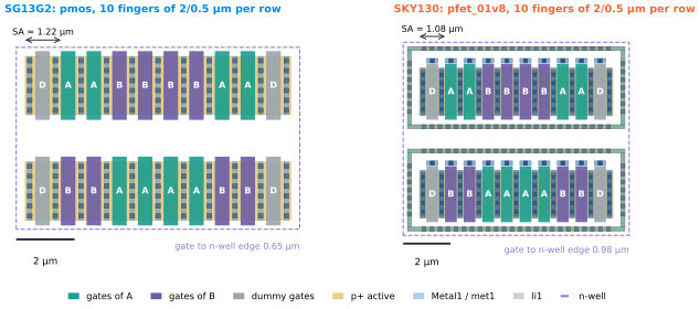
pmos, Magic pfet_01v8 with its tap ring), assigned D ABBA D and D BAAB D in 2-finger units that share their drain. Placement only: the routing and the SG13G2 well tap are left out.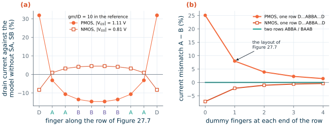
Worked example 27.3 · Trench stress in a one-row ABBA, by hand and by simulation
Geometry. Finger \(i\) (0 to 9) of the SKY130 row has SA = 0.29 + 0.79 \(i\) µm and SB = 0.29 + 0.79 (9 − \(i\)) µm, with L = 0.5 µm. Eq. (27.7) gives Inv = 0.898, 0.636, 0.533 and 0.493 µm⁻¹ for fingers 1 to 4 (fingers 5 to 8 mirror them). A, fingers 1, 2, 7, 8, averages 0.767 µm⁻¹; B, fingers 3 to 6, averages 0.513 µm⁻¹: a difference of 0.254 µm⁻¹.
Threshold difference. \(K_{stress} = 1 + 0.2/2\) = 1.10. PMOS: \(\Delta V_{TH} = 3.29 \times 10^{-8} \times 2.54 \times 10^{5}/1.10\) = 7.6 mV, smaller in magnitude for A. NMOS: \(9.8 \times 10^{-9} \times 2.54 \times 10^5/1.10\) = 2.3 mV, larger for A. Between fingers 1 and 4 alone the hand values are 12.1 and 3.6 mV; the simulation, comparing the gate voltages at which the two fingers carry the same current, gives 12.1 and 3.6 mV.
Current mismatch. At gm/ID = 10, \(\Delta I/I \approx (g_m/I_D)\,\Delta V_{TH}\): +7.6 % for the PMOS pair and −2.2 % for the NMOS pair. The simulated rows give +8.0 % and −2.2 % (Figure 27.8b, one dummy).
Result. In SKY130’s models, the PMOS pair of Figure 27.7 has a systematic threshold difference of 7.6 mV, almost twice its random σ of 4.2 mV (4 µm² of gate per device, \(A_{VT}\) = 8.4 mV·µm), although its centroids coincide. LOD is an even function along the row, exactly like the \(x^2\) term of Eq. (27.5), and one-row ABBA does not cancel it. The second row, BAAB, gives B the outer positions and cancels it exactly; more dummy fingers only reduce it (2.3 % with three per end). In SG13G2, the same calculation returns zero, because the model has no stress terms.
Common pitfall · A common centroid that trench stress breaks
A designer who puts an input pair or a mirror on one long active area as ABBA, with one dummy finger at each end, has done everything Section 27.3 asks and may still find a few millivolts of offset that no Monte Carlo predicted. Neither the schematic simulation (no SA, SB) nor the post-layout netlists of these PDKs (Chapter 15) include the stress, and SG13G2’s models would not show it even if they did. Cancel it by construction: give each unit its own active area, so that every unit sees the same SA and SB; or use the two-row ABBA/BAAB; or add enough dummy fingers that the active fingers sit where the stress has flattened out. Separate active areas cost the shared diffusion’s capacitance advantage and shift every device’s current away from the schematic value (in SKY130 a finger with SA = 0.29 and SB = 1.08 µm carries 55 % more current as a PMOS and 13 % less as an NMOS than the model without SA, SB), but they shift A and B equally. The course OTA of Chapter 15 gives each unit its own active area.
Well proximity
The other layout-dependent effect of Chapter 15 comes from the high-energy well implant: ions that scatter off the edge of the resist mask land in the silicon just inside the well, so a transistor within a micrometre or two of the well edge has a higher threshold than one far from it [84]. Its magnitude depends on the distance SC from the gate to the well edge, and BSIM4 and PSP both have terms for it. Neither PDK simulates it. SKY130’s nfet_01v8 and pfet_01v8 cards contain none of BSIM4’s well-proximity parameters and their subcircuits pass only SA, SB and SD; SG13G2’s PSP cards set the well-proximity coefficients (KVTHOWEO, KUOWEO) to zero and its subcircuits pass none of the distances [19, 14]. The generators of Figure 27.7 put the outermost gate 0.65 µm (SG13G2) and 0.98 µm (SKY130) from the n-well edge, close enough for the effect to be present on silicon. For matched devices:
- keep the well edge several micrometres from every active gate where the area allows, and at the same distance on all sides of an array [61];
- let dummy devices, not active ones, sit next to the well edge;
- give the two halves of a differential circuit mirror-symmetric wells, never a well that is wider on one side.
Gate density, metal and fill
Etching and polishing depend on the density of the pattern around a structure. A gate with neighbours on both sides etches to a slightly different length from a gate at the end of a row, which is a reason for dummy gates beyond the trench-stress one. The same applies to metal: dense routing over one device of a pair, or automatically inserted fill over one and not the other, changes the stress and the hydrogen that reaches the gate oxide during processing [61]. Route over matched devices only when every device sees the same metal, and keep fill out of a matched array or make it symmetric; SG13G2’s generators already mark inductors as no-fill areas (Chapter 26), and the same markers can be drawn over a matched array.
SG13G2 vs SKY130 · What the models know about layout
Effect SG13G2 models SKY130 models Random mismatch of MOS, resistors, MIM yes ( mm_ok=1,*_mismatchsections)yes ( tt_mm,mc)Random mismatch of MOM capacitors no no Trench stress (LOD, SA/SB) no (all coefficients zero) yes, threshold term Well proximity (SC) no no Gradients, package stress no no So in SKY130 you can simulate a matched row with the SA and SB of each finger, as in Figure 27.8, and you should; in SG13G2 you cannot, and the layout must cancel LOD by construction. In neither PDK will a simulation reveal a well-proximity or a gradient error.
27.6 Dummies, symmetry and routing
What dummies do and how to connect them
A dummy is a copy of a unit that takes no part in the circuit. It exists to make the edge of an array look like its interior, and so the questions are how far the edge effects reach and what potential the dummy should sit at [61]:
- Lithography and etch effects are short-range: one dummy unit, or a narrower dummy strip of the same layer at the same spacing, covers them.
- Trench stress reaches micrometres: in a row on a shared active area it takes several dummy fingers (Figure 27.8b), or a separate active area per unit.
- Well proximity is strongest within a micrometre or two of the well edge, with a tail beyond [84]: dummies between the active devices and the well edge push the edge away.
Connect every dummy. A floating poly or metal plate can charge during processing and later couple noise or shift a neighbour. Dummy transistors go off: an NMOS dummy with gate, source and drain on ground, a PMOS dummy on the supply. Dummy resistors and capacitors go to a quiet, low-impedance node, usually analog ground, and never to a node whose noise would couple into the matched devices or whose load the dummies’ capacitance would disturb. The resistor ring of Figure 27.5 and the shorted dummy ring of Figure 27.6 do this.
Symmetry of the whole circuit
Matching does not end at the devices. A differential circuit has two halves, and everything attached to them, wires, vias, contacts, neighbours, should be mirror images [61]:
- Wires that carry current add resistance in series with a device. In a source-coupled pair with a tail of 20 µA, 10 µA flows in each source; an extra 50 µm of 0.5 µm Metal1 (110 mΩ/□ in SG13G2, Chapter 15’s Table 15.3) is 11 Ω, which adds 110 µV to that side’s gate-source voltage: a fifth of the random σ of a good pair. Route the two sources to a common point with equal lengths and equal numbers of vias, or use a separate sense connection (a Kelvin connection) where a precise voltage is needed.
- Wires that carry no current still add capacitance. In capacitor arrays this changes the ratios; give every unit the same stub, as in Figure 27.6, and make every crossing happen for all matched wires alike.
- Neighbours. A digital line along one side of a pair couples into that side only. Keep switching signals away, or shield the matched devices on all sides equally.
Guard rings and quiet surroundings
Matched devices are often also sensitive ones: the input pair of an amplifier, the reference branch of a mirror. Surround them with a substrate-tap ring (NMOS) or a well-tap ring (PMOS), as Chapter 24 requires for latch-up anyway; the ring fixes the local substrate potential that all the matched devices share and collects carriers injected by neighbouring circuits. Make the ring symmetric around the array, so that every device sees the same distance to its taps. The SKY130 generator draws such a ring around each row of Figure 27.7.
What Chapter 15’s OTA does, and what it would gain
The course OTA of Chapter 15 uses an ABBA input pair of two units per device, each unit on its own active area, with a dummy at each row end. By Figure 27.4 this cancels both linear gradients and leaves \(2hp^2\) of curvature along the row; by Figure 27.8 its separate active areas make LOD equal for A and B. Drawn as two rows ABBA/BAAB with four units per device, the pair would cancel the curvature as well, at the cost of one more row and a little more routing; Section 27.3’s insight box applies.
27.7 A checklist for matched devices
Before a matched layout goes to verification, walk through these questions. Most of them cannot be checked by DRC or LVS, and none of the effects behind them appears in a post-layout simulation of these PDKs except the wiring parasitics.
All matched devices
- Is each device built from identical units of one cell, in the same orientation, with current in the same direction?
- Is the random part large enough? Size from Table 27.1 (or Chapter 13 for transistors) for the σ the circuit needs, with margin for the systematic part.
- Do the centroids coincide, and for four or more units per device, do the second moments too (Figure 27.4)? Is a large array split into small common-centroid groups?
- Do dummies surround the array, at the same pitch and of the same shape, and are they connected to a quiet node?
- Is the array away from heat sources, die edges and corners, and on an axis of symmetry of the heat sources where possible?
- Is the routing symmetric: equal lengths and vias in current-carrying paths, the same crossings and neighbours for both halves, no unrelated metal or fill over only part of the array?
Resistors
- Same width and segment length throughout, straight segments joined in metal, heads in equal numbers, current flowing both ways in each resistor, jumpers outside the bodies (Figure 27.5)?
Capacitors
- Whole numbers of unit capacitors, a dummy ring, top plate on the sensitive node, identical stubs for every unit (Figure 27.6)?
Transistors
- Every unit on its own active area, or two-row ABBA/BAAB, or enough dummy fingers that LOD has flattened out? In SKY130, simulate the fingers with their SA and SB as in Figure 27.8.
- Matched gates several micrometres from the well edge, with the same distance on all sides, and dummies next to the edge?
- A symmetric guard ring around the matched group?
Try it · Change a pattern, add dummies
In
tools/layout/ch27/match_layouts.py, setRES_PATTERN = "DAAAABBBBD"and rerunpython3 tools/layout/ch27/match_layouts.py build exportandpython3 tools/figs/ch27_matching.py res: the jumpers get simpler, and Figure 27.4 tells you that the array now has four pitches of linear error. Then try your own C-DAC assignment: editCCAintools/figs/ch27_matching.py(for example move C1 and C0 to two corners) and runpython3 tools/figs/ch27_matching.py cdacto see the share errors change. Finally, intools/figs/_ch27_sim.py, extendNDto 8 and rerunpython3 tools/figs/_ch27_sim.py sky130andpython3 tools/figs/ch27_matching.py lod: how many dummy fingers per end bring the PMOS mismatch below the random σ of 4.2 mV, that is below about 4 % of current at gm/ID = 10?
- Mismatch has a random part, which falls only with area, and a systematic part, which a layout can cancel. Random coefficients from the PDK models: \(A_R\) = 2.78 %·µm (SG13G2
rppd) and about 4.5 %·µm (SKY130res_high_po); \(A_C\) = 1.41 and 3.90 %·µm for the MIM capacitors. For σ = 0.1 %, SKY130 needs 2.7 times the resistor area and ten times the capacitance of SG13G2.- A gradient adds \(g\,d\) for centroids a distance \(d\) apart; for side-by-side devices it overtakes the random part at a few tens of micrometres. Eq. (27.5) grades any placement: coinciding centroids cancel linear gradients, equal second moments cancel curvature. ABBABAAB and ABBA/BAAB cancel both; the quad AB/BA keeps a saddle term.
- A 100 mW heat source 200 µm away puts 40 µV on a side-by-side NMOS pair and well under a microvolt on a common-centroid one; thermal gradients matter only near power devices.
- In a capacitor array, every capacitor of two or more units can be made immune to linear gradients; for a 4-bit array the random part dominates, but the breakeven gradient halves with every bit.
- SKY130’s models contain trench stress: on a shared active area, a one-row PMOS ABBA with one dummy per end has a systematic 7.6 mV (8 %) mismatch at gm/ID = 10. Separate active areas, two-row ABBA/BAAB or several dummies remove it. SG13G2’s models contain no stress terms, and neither PDK models well proximity: cancel both by construction.
Further reading
- R. A. Hastings, The Art of Analog Layout [61], Chapter 8 (matching of resistors and capacitors: causes of mismatch, the four rules of common-centroid layout, thermal and stress gradients, rules by level of accuracy) and Sections 13.2–13.3 (matching of MOS transistors, including proximity effects).
- M. J. M. Pelgrom, A. C. J. Duinmaijer and A. P. G. Welbers [75]: the area law and the distance term of Eq. (27.3), measured.
- J.-B. Shyu, G. C. Temes and F. Krummenacher [111]: random errors of matched capacitors and current sources, and how edge and area terms combine.
- P. G. Drennan, M. L. Kniffin and D. R. Locascio [84] on well proximity and trench stress in analog design, and K.-W. Su et al. [83] for the stress model of Eq. (27.7).
- The mismatch sections of the PDKs’ model libraries,
cornerRES.lib,cornerCAP.libandcornerMOSlv.libfor SG13G2 [14] and thett_mmsection and*__mismatchfiles of SKY130 [19]: they state exactly which random terms each device carries.