Chapter 13
Noise and Mismatch
Two random effects limit every analog circuit: noise, which changes from moment to moment, and mismatch, which is frozen in when the chip is made. Both are predictable from a handful of device constants, and both can be designed for with the same levers: gm/ID, area and current.
- Describe thermal, shot and flicker noise, and model the noise of a MOSFET with two numbers, \(\gamma\) and \(K_f'\).
- Simulate noise in ngspice, refer it to the input, and integrate it over a bandwidth.
- Compute the input-referred noise of a common-source stage and of the 5T OTA, and choose gm/ID and area to reduce it.
- Explain kT/C noise and why it does not depend on the resistor.
- Extract Pelgrom’s mismatch constants from Monte Carlo simulation in both PDKs, and predict the offset of a differential pair and an OTA.
Contents
13.1 Noise sources
Every resistor and transistor in a circuit is made of charge carriers in random thermal motion. The current they carry is therefore not perfectly smooth: it fluctuates around its average by a tiny amount that no circuit trick can remove. We call this fluctuation noise. It sets the smallest signal an amplifier can handle, just as the supply sets the largest, so the ratio of the two, the dynamic range, is fixed by noise.
Noise is random, so we cannot say what its value will be at any instant. We describe it instead by its power spectral density (PSD), the mean-square value per hertz of bandwidth, \(S_v(f)\) in V²/Hz (or \(S_i(f)\) in A²/Hz). Datasheets and simulators often quote its square root, the noise density in V/√Hz. The total, or integrated, noise in a band is the area under the PSD,
\[\overline{v_n^2} = \int_{f_1}^{f_2} S_v(f)\,df, \qquad v_{n,\mathrm{rms}} = \sqrt{\overline{v_n^2}}. \tag{13.1}\]Noise sources that come from different physical processes are uncorrelated, so their mean-square values (not their rms values) add. Three kinds of noise matter in CMOS circuits [51, 53].
-
Thermal noise. The random motion of carriers in any resistance \(R\) produces an open-circuit voltage with a flat (“white”) PSD,
\[S_v = 4kTR \quad\text{or, as a current,}\quad S_i = \frac{4kT}{R}, \tag{13.2}\]where \(k\) is Boltzmann’s constant and \(T\) the absolute temperature. At 27 °C, \(4kT = 1.66\times10^{-20}\) J, so a 1 kΩ resistor has 4.07 nV/√Hz. Thermal noise needs no current: it is present in a resistor sitting on a shelf.
- Shot noise. A current made of discrete charges crossing a barrier, such as a pn junction or a transistor in weak inversion, has \(S_i = 2qI\). It appears in diodes, bipolar transistors and gate leakage.
- Flicker noise. Carriers are trapped and released by defects at the silicon–oxide interface, so the number of carriers in a MOSFET channel fluctuates slowly. The resulting PSD rises towards low frequencies, roughly as \(1/f\), which is why it is also called 1/f noise. It dominates below a frequency called the flicker corner and is the reason why precision circuits avoid MOSFETs at the input or chop them (Section 13.4).
13.2 MOSFET noise
Thermal noise of the channel
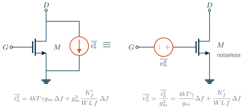
The channel of a MOSFET in saturation is a resistive sheet of charge, and its thermal noise appears as a noise current between drain and source (Figure 13.1, left):
Key equation · MOSFET drain-current noise
\[S_{id} = 4kT\gamma g_m \;+\; g_m^2\,\frac{K_f'}{WL\,f}, \qquad\text{or at the gate:}\qquad S_{vg} = \frac{S_{id}}{g_m^2} = \frac{4kT\gamma}{g_m} + \frac{K_f'}{WL\,f}. \tag{13.3}\]\(\gamma\) is the thermal noise factor and \(K_f'\) the flicker coefficient of the process. Both terms of \(S_{vg}\) fall as the transistor gets “bigger”: more \(g_m\) for the thermal term, more gate area for the flicker term.
For a long-channel device in strong inversion, theory gives \(\gamma = 2/3\); in weak inversion the channel current is a diffusion current with shot noise \(2qI_D\), which gives \(\gamma = n/2 \approx 0.65\) [58, 59]. Short-channel devices show larger values. Because \(S_{vg} \propto 1/g_m\), the only way to lower the thermal noise of a transistor is more transconductance, which costs current. This is the first and most important noise lever.
Flicker noise
The second term of Eq. (13.3) is the flicker noise, referred to the gate. Its PSD is inversely proportional to the gate area \(WL\), because a larger gate averages over more traps. We characterize each process by the single constant
\[K_f' = S_{vg}(f)\cdot f\cdot WL \qquad [\mathrm{V^2\,\mu m^2}], \tag{13.4}\]which is the input-referred flicker PSD at 1 Hz of a 1 µm² transistor. Older textbooks write it as \(K/(C_{ox}WLf)\); we fold \(C_{ox}\) into \(K_f'\) because both PDKs model flicker noise with bias-dependent expressions (PSP’s NFA, NFB, NFC in SG13G2; BSIM4’s NOIA, NOIB, NOIC in SKY130) whose result is easiest to read off a simulation [73, 14, 19]. Since the models do not follow exactly \(1/f\), we evaluate \(K_f'\) at 1 kHz.
Setting the two terms of Eq. (13.3) equal gives the flicker corner:
\[f_c = \frac{K_f'\,g_m}{4kT\gamma\,WL}. \tag{13.5}\]At a fixed \(g_m/I_D\) the current density \(I_D/W\) is fixed, so \(g_m/W\) is fixed, and Eq. (13.5) says \(f_c \propto 1/L\) times \(g_m/W\). In strong and moderate inversion \(g_m/W\) itself falls roughly as \(1/L\), so the flicker corner falls roughly as \(1/L^2\), independently of \(W\).
What the models say
Figure 13.2 shows the input-referred noise of single transistors simulated with each PDK’s own noise models: W = 5 µm, \(g_m/I_D = 15\) V⁻¹, \(\lvert V_{DS}\rvert = V_{DD}/2\). Panel (a) has the textbook shape: a 1/f slope at low frequency and a white floor above the corner. Panel (b) shows the corner for ten lengths. It falls by a factor of 100 to 1700 between L = 0.18 µm and 5 µm, close to the \(1/L^2\) guide for most devices; the SKY130 PMOS falls more slowly because its \(K_f'\) grows with length.
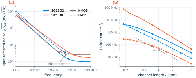
Figure 13.3 shows how the two noise constants depend on the inversion level at L = 1 µm, and Table 13.1 collects the values used in the rest of this chapter.
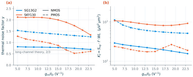
Table 13.1. Noise constants from the PDK models at gm/ID = 15 V−1 (W = 5 µm, |VDS| = VDD/2, tt, 27 °C). Kf′ in µV²·µm², evaluated at 1 kHz.
| Quantity | SG13G2 NMOS | SG13G2 PMOS | SKY130 NMOS | SKY130 PMOS |
|---|---|---|---|---|
| \(\gamma\), L = 0.5 / 1 / 2 µm | 0.79 / 0.78 / 0.76 | 1.36 / 1.37 / 1.37 | 1.89 / 2.00 / 2.22 | 0.86 / 0.87 / 0.82 |
| \(K_f'\), L = 0.5 / 1 / 2 µm | 187 / 210 / 223 | 556 / 577 / 591 | 753 / 835 / 799 | 114 / 178 / 193 |
| \(f_c\), L = 0.5 / 1 / 2 µm | 1.39 MHz / 436 kHz / 123 kHz | 686 / 185 / 48 kHz | 9.2 / 1.9 / 0.38 MHz | 128 / 50 / 15 kHz |
| \(\sqrt{S_{vg}}\) at 1 kHz, 1 µm² | 0.46 µV/√Hz | 0.76 µV/√Hz | 0.91 µV/√Hz | 0.42 µV/√Hz |
SG13G2 vs SKY130 · Which input device is quieter?
The folklore says “PMOS has less flicker noise than NMOS, so use a PMOS input pair”. In SKY130 that holds strongly: the NMOS has 4.7 times the \(K_f'\) of the PMOS at L = 1 µm, and its corner at L = 0.18 µm is 74 MHz. In SG13G2 it is the other way round: the PSP flicker parameters give the PMOS 2.7 times the \(K_f'\) of the NMOS (NFALW is 2.2×10²⁶ against 7.6×10²⁵ in the model file). The thermal factors also differ: SKY130’s NMOS model (BSIM4,
tnoimod = 1) gives \(\gamma \approx 2\) even at L = 5 µm, three times the long-channel value, while SG13G2’s NMOS stays near 0.8. Choose the input device type from your PDK’s numbers, not from folklore, and remember that model noise parameters are fits to measured wafers with their own uncertainty. SKY130’s flicker noise also falls as \(1/f^{0.84}\) rather than \(1/f\) (model parameter EF = 0.84), which matters when you extrapolate over decades.
Simulating noise in ngspice
The .noise analysis linearizes the circuit at its operating point, like .ac, and adds up every noise generator in every device, each transferred to a chosen output [36]. It needs an output node and an input source; it reports the output noise and the same noise divided by the gain from that source, the input-referred noise. To see a transistor’s drain-current noise directly, we sense the drain current with a 0 V source and turn it into a voltage with a 1 Ω current-controlled voltage source. The output then reads \(\sqrt{S_{id}}\) in A/√Hz, and the gain from the gate source is \(g_m\):
* Drain-current noise of one NMOS: W = 5 um, L = 1 um, gm/ID = 15 (VGS from the gm/ID table)
.lib cornerMOSlv.lib mos_tt
Vd d 0 0.6
Vg g 0 dc 0.315 ac 1
XM1 dd g 0 0 sg13_lv_nmos W=5u L=1u ng=1 m=1
* sense the drain current and convert it to a voltage, 1 V per A
Vs d dd 0
Hs out 0 Vs 1
.control
* last argument 1: also report every noise generator separately
noise v(out) Vg dec 10 1 1e9 1
setplot noise1
wrdata spectra.txt inoise_spectrum onoise_spectrum
setplot noise2
print inoise_total onoise_total
.endc
.end
* Drain-current noise of one NMOS: W = 5 um, L = 1 um, gm/ID = 15 (VGS from the gm/ID table)
.lib "$PDK_ROOT/sky130A/libs.tech/ngspice/sky130.lib.spice" tt
Vd d 0 0.9
Vg g 0 dc 0.682 ac 1
XM1 dd g 0 0 sky130_fd_pr__nfet_01v8 W=5 L=1 nf=1
* sense the drain current and convert it to a voltage, 1 V per A
Vs d dd 0
Hs out 0 Vs 1
.control
* last argument 1: also report every noise generator separately
noise v(out) Vg dec 10 1 1e9 1
setplot noise1
wrdata spectra.txt inoise_spectrum onoise_spectrum
setplot noise2
print inoise_total onoise_total
.endc
.end
Common pitfall · Reading the wrong noise plot
One
noisecommand creates two plots:noise1holds the spectra (inoise_spectrum,onoise_spectrumand, with the last argument set, one vector per noise generator) andnoise2holds the integrated totals over the analysis range. The plot that is current after the analysis isnoise2, so a plainwritesaves only the integrated numbers. Select the plot first, as above, or name both in one command,write out.raw noise1.all noise2.all, which is what our scripts do. Also note that ngspice reports densities (V/√Hz) and integrated rms values (V), not PSDs: square them before adding. Our figure scripts,tools/figs/ch13_noise.pyand its helper module, wrap all of this, including several noise analyses in one run.
13.3 Input-referred noise
A circuit with many noise sources is described most usefully by a single input-referred noise source: the noise at the input of a noiseless copy of the circuit that gives the same output noise,
\[S_{v,in}(f) = \frac{S_{v,out}(f)}{\lvert A(f)\rvert^2}. \tag{13.6}\]It can be compared directly with the input signal, and it does not depend on the load or the bandwidth of the stage that follows. For a common-source stage with transistor \(M_1\) and a PMOS current-source load \(M_2\), both drain-current noises flow into the output node. Referring each to the gate of \(M_1\) with Eq. (13.3):
Key equation · Input-referred noise of a common-source stage
\[S_{v,in} = \frac{4kT}{g_{m1}}\left(\gamma_1 + \gamma_2\frac{g_{m2}}{g_{m1}}\right) + \frac{K_{f1}'}{W_1L_1 f} + \left(\frac{g_{m2}}{g_{m1}}\right)^2\frac{K_{f2}'}{W_2L_2 f}. \tag{13.7}\]The load adds noise in proportion to \(g_{m2}/g_{m1} = (g_m/I_D)_2/(g_m/I_D)_1\), because both carry the same current. Bias current sources at low gm/ID (strong inversion), and amplifying devices at high gm/ID.
Worked example 13.1 · Noise of the Chapter 6 common-source stage
Take the common-source stage of Worked example 6.1 (\(I_D\) = 41.9 µA, \(g_{m1}\) = 628 µS, \(g_m/I_D = 15\); SG13G2 W/L = 18.05/0.75 µm, SKY130 4.62/0.18 µm) and replace its ideal current source by a PMOS load at \(g_m/I_D = 8\), L = 2 µm, which the gm/ID tables size to W = 36.6 µm (SG13G2) and 43.6 µm (SKY130). Then \(g_{m2}/g_{m1} = 8/15 = 0.53\).
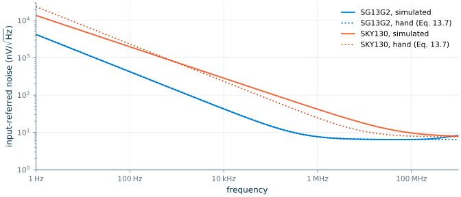
Thermal floor. With the single-device values at each length (SG13G2 \(\gamma_1 = 0.78\), \(\gamma_2 = 1.47\); SKY130 \(\gamma_1 = 1.68\), \(\gamma_2 = 0.97\)), Eq. (13.7) gives \(S_{v,in} = \frac{1.66\times10^{-20}}{628\ \mu\mathrm{S}}\,(0.78 + 1.47\times0.53) = 4.13\times10^{-17}\ \mathrm{V^2/Hz}\), or 6.43 nV/√Hz in SG13G2, and 7.61 nV/√Hz in SKY130. The load raises the SG13G2 floor from 4.55 to 6.43 nV/√Hz: it doubles the noise power.
Flicker noise at 1 kHz. In SG13G2, \(K_{f1}' = 202\) µV²µm² over 13.5 µm² gives 122 nV/√Hz from \(M_1\), and the load (\(K_{f2}'\) = 778 µV²µm² over 73.2 µm², weighted by \(0.53^2\)) adds 55 nV/√Hz: 134 nV/√Hz in total. In SKY130 the tiny \(M_1\) (0.83 µm², \(K_f'\) = 455 µV²µm²) alone gives 740 nV/√Hz, and the load is negligible. The SG13G2 corner, from the total flicker and thermal terms, is at 434 kHz.
Simulation. Figure 13.4 compares Eq. (13.7) with ngspice. The thermal floors are 6.39 and 7.62 nV/√Hz (within 1 % of the hand values) and the 1 kHz values 134 and 749 nV/√Hz (within 2 %). The SG13G2 corner is at 441 kHz (hand 434 kHz). In SKY130 the hand line is only right near 1 kHz, where we measured \(K_f'\): the model’s \(1/f^{0.84}\) slope puts the real corner at 56 MHz, six times the 9.4 MHz that a \(1/f\) extrapolation predicts.
The worked example also shows that the two designs of Chapter 6, which had the same gain and bandwidth, are very different in noise. The SKY130 transistor was short and narrow to keep its capacitance small; with 16 times less gate area, it has 5.6 times more flicker noise at 1 kHz.
13.4 Noise of the OTA
Our amplifier for the rest of this chapter is the five-transistor OTA that Chapter 10 designed for the course load and bandwidth (Figure 13.5). Its NMOS input pair runs at \(g_m/I_D = 16\) with L = 1 µm and its PMOS mirror at 10 with L = 1 µm, each built from three fingers of about 5 µm. Each side carries 20 µA, so \(g_{m1}\) = 320 µS, a margin above the \(2\pi\cdot 20\ \mathrm{MHz}\cdot 2\ \mathrm{pF} = 251\) µS that the specification requires; the tail transistor mirrors four times a 10 µA reference. In SG13G2 the pair is 13.68/1 µm and the mirror 14.85/1 µm, in SKY130 16.41/1 µm and 17.28/1 µm. We simulate exactly Chapter 10’s netlists, with the input at its common-mode level of 0.7 V (SG13G2) and 1.1 V (SKY130). Chapter 10 found a GBW of 23.8 and 24.5 MHz and DC gains of 26.5 and 41.7 dB; the SG13G2 gain is far below the course’s 60 dB, which is why the course project uses two stages (Chapter 12).
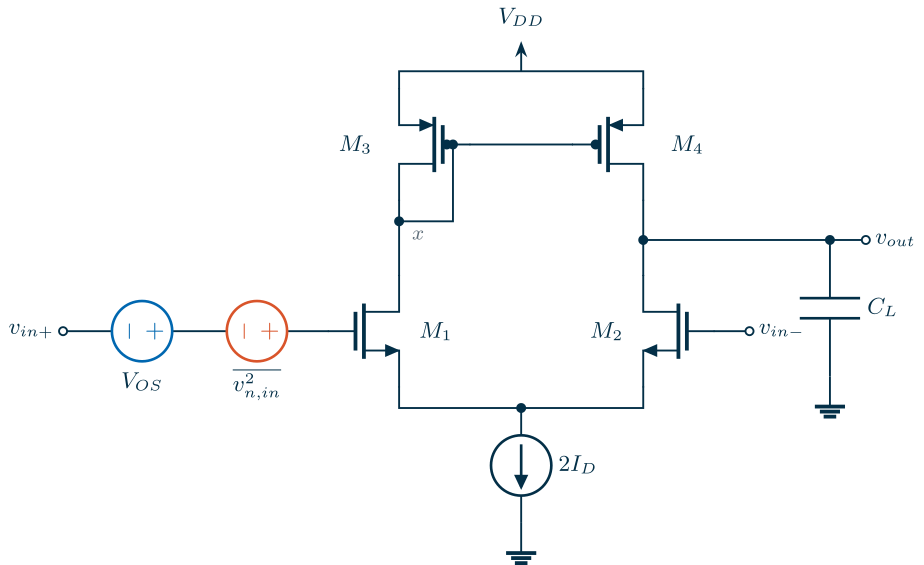
Each of the four transistors injects its drain-current noise into the output. \(M_1\) and \(M_2\) are input devices; \(M_3\)’s noise is copied to the output by the mirror, and \(M_4\)’s goes there directly. Referring all four to the input:
Key equation · Input-referred noise of the 5T OTA
\[S_{v,in} = \underbrace{\frac{2\cdot 4kT}{g_{m1}}\left(\gamma_1 + \gamma_3\frac{g_{m3}}{g_{m1}}\right)}_{\text{thermal}} + \underbrace{\frac{2}{f}\left(\frac{K_{f1}'}{W_1L_1} + \left(\frac{g_{m3}}{g_{m1}}\right)^2\frac{K_{f3}'}{W_3L_3}\right)}_{\text{flicker}}. \tag{13.8}\]The factor 2 is the price of a differential pair: two transistors contribute where a single-ended stage has one.
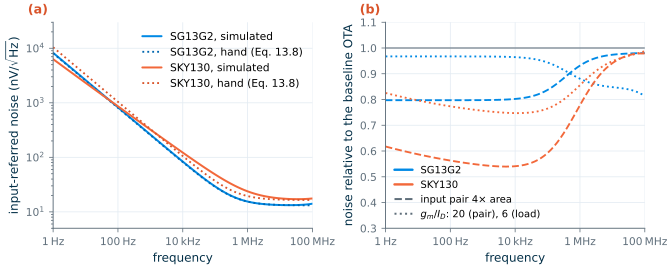
With the constants of each device at its own bias, Eq. (13.8) predicts a thermal floor of 13.1 nV/√Hz in SG13G2 and 16.5 nV/√Hz in SKY130; the simulated white parts are 13.1 and 16.4 nV/√Hz. At 1 kHz it predicts 256 and 330 nV/√Hz against 261 and 323 nV/√Hz simulated (Figure 13.6a). Here the PDKs differ sharply. In SG13G2 the mirror contributes 53 % of the flicker noise at 1 kHz, because its PMOS has 3.4 times the \(K_f'\) of the NMOS pair (680 against 203 µV²µm²); in SKY130 it contributes only 8 %.
The design levers
Figure 13.6b tries the levers that Eq. (13.8) offers, while keeping \(g_{m1}\), and therefore the GBW, fixed.
- Gate area (dashed). Doubling \(W_1\) (six fingers instead of three) and \(L_1\) keeps \(g_m/I_D\) and the current, and quadruples the gate area. The flicker noise of the pair falls by four in power, a factor of two in density. In SKY130, where the pair dominates, the OTA’s noise at 1 kHz falls from 323 to 176 nV/√Hz. In SG13G2 it falls only from 261 to 208 nV/√Hz, because the unchanged mirror is now 80 % of the flicker noise: in this PDK the area belongs in the mirror. The white floor does not move. The cost is four times the input capacitance, which loads the previous stage.
- gm/ID (dotted). Biasing the pair at 20 V⁻¹ and the mirror at 6 V⁻¹ shrinks \(g_{m3}/g_{m1}\) from 0.63 to 0.30, and the current falls from 20 to 16 µA per side, because \(g_{m1}\) now costs less current. The white floor drops from 13.1 to 10.9 nV/√Hz in SG13G2 and from 16.4 to 15.3 nV/√Hz in SKY130 (Eq. (13.8) predicted 14.4 nV/√Hz, 6 % lower). The 1/f noise falls by 24 % in SKY130 but only by 3 % in SG13G2: at gm/ID = 6 the mirror is only 3.9 µm wide, and its smaller area undoes most of the benefit of its smaller weight \((g_{m3}/g_{m1})^2\). The price is a larger pair, less output swing (the mirror’s \(V_{SG}\) rises from 0.52 to 0.67 V in SG13G2) and a lower \(V_{DS}\) on the input pair.
- Current. To halve the thermal noise density at the same gm/ID you must quadruple \(g_m\) and hence the current. Noise is paid for in power.
- Device type. Using a PMOS input pair is the classic cure for flicker noise, and in SKY130 it would cut \(K_f'\) by four. In SG13G2 it would make it worse (Table 13.1).
The two-stage OTA of Chapter 12, simulated in the same test bench, has 428 nV/√Hz (SG13G2) and 370 nV/√Hz (SKY130) at 1 kHz, and 25 and 31 nV/√Hz at 1 MHz. Eq. (13.8) applies to its first stage unchanged. That stage carries only 10 µA per side, which raises the white floor, and its PMOS mirror is short (L = 0.5 µm), which in SG13G2 makes the mirror’s flicker term dominant despite an input pair of 55 µm².
What this means for your design
Decide which noise matters. For audio and sensor interfaces (below about 100 kHz), flicker noise dominates and gate area of the input pair is the main lever; put the extra area in L as well as W, because \(f_c \propto 1/L^2\). For wideband circuits, the white floor dominates and gm of the input pair is the lever, which you pay for in current. In both cases make the load’s \(g_m\) small compared with the pair’s: low gm/ID and long L for current sources. When even large devices cannot reach the flicker floor you need, chopping or correlated double sampling move the signal away from DC; they are beyond this course, see Sansen [62].
Integrated noise of a closed loop
Connected as a unity-gain buffer, the OTA has a single-pole bandwidth \(f_u = g_{m1}/(2\pi C_L)\), and its noise bandwidth is \((\pi/2)f_u\). Integrating the thermal part of Eq. (13.8) over it gives
\[\overline{v_{n,out}^2} = \frac{2kT}{C_L}\left(\gamma_1 + \gamma_3\frac{g_{m3}}{g_{m1}}\right). \tag{13.9}\]The transconductance has cancelled: a larger \(g_{m1}\) lowers the noise density but widens the bandwidth by the same factor. For Chapter 10’s OTA, Eq. (13.9) gives 83.2 µV rms (SG13G2) and 104.2 µV rms (SKY130). ngspice gives 77.5 and 99.9 µV for the white part, and 85.3 and 116 µV including the flicker noise down to 1 Hz. The result has the form \(kT/C\) times a factor, which brings us to the next section.
13.5 kT/C noise
Consider a switch, with on-resistance \(R_{on}\), charging a capacitor \(C\) (Figure 13.7). The switch’s thermal noise, Eq. (13.2), is shaped by the RC low-pass filter, and the total noise on the capacitor is
\[\overline{v_n^2} = \int_0^\infty \frac{4kTR_{on}}{1 + (2\pi f R_{on} C)^2}\,df = \frac{kT}{C}. \tag{13.10}\]The resistance has cancelled again. A larger \(R_{on}\) makes more noise per hertz but a narrower bandwidth, and the two effects balance exactly. The same answer follows from thermodynamics: a capacitor in thermal equilibrium stores an average energy of \(\tfrac12 kT\), so \(\tfrac12 C\overline{v^2} = \tfrac12 kT\) [51, 52]. When the switch opens, this noise voltage is frozen on the capacitor as a random sample. kT/C noise sets the minimum capacitor size in every sampled-data circuit: switched-capacitor filters, sample-and-hold circuits and ADCs.
Table 13.2. kT/C noise at 27 °C.
| \(C\) | 10 fF | 100 fF | 1 pF | 2 pF | 10 pF |
|---|---|---|---|---|---|
| \(\sqrt{kT/C}\) | 644 µV | 204 µV | 64.4 µV | 45.5 µV | 20.4 µV |
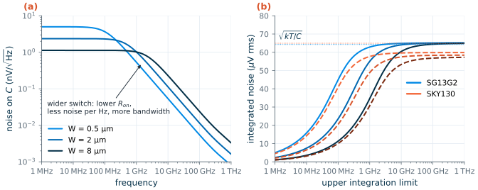
Figure 13.7 checks Eq. (13.10) with PDK devices: a minimum-length NMOS switch, with its gate at \(V_{DD}\), and a 1 pF MIM capacitor (SG13G2 cap_cmim, 25.8 × 25.8 µm, 1.003 pF; SKY130 cap_mim_m3_1, 22 × 22 µm, 0.983 pF). Making the switch 16 times wider lowers the noise density and stretches the bandwidth from 108 MHz to 2.1 GHz, but the integrated noise on the SG13G2 capacitor stays at 65.0 µV for every width, 1 % above \(\sqrt{kT/C} = 64.3\) µV.
SG13G2 vs SKY130 · Switch noise at zero drain voltage
In SKY130 the integrated noise settles at 57–60 µV, 8–12 % below \(\sqrt{kT/C}\). A switch with no voltage across it is in thermal equilibrium, so physics requires exactly \(kT/C\), and an ideal resistor in the same netlist does give it (65.0 µV). The BSIM4 thermal-noise model used by SKY130 (
tnoimod = 1) is fitted for amplifying transistors in saturation; at \(V_{DS} = 0\) it gives only about 0.8 × \(4kT/R_{on}\). SG13G2’s PSP model gets it right. For sampled circuits in SKY130, trust \(kT/C\), not the simulator. A second trap: both MIM models contain a small series resistance (55 mΩ in SG13G2), whose white noise integrated up to 1 THz adds tens of microvolts. Measure the noise across the capacitor itself, or stop the integration at a realistic bandwidth.
13.6 Mismatch and Pelgrom’s law
Two transistors drawn identically, side by side, are never quite identical. The number and position of the dopant atoms under each gate are random, the oxide thickness and the edges of the gate vary on an atomic scale, and so do the mobility and the trapped charge. Each transistor therefore has its own threshold voltage \(V_{TH}\) and current factor \(\beta = \mu C_{ox}W/L\). The differences are random, frozen in at fabrication, and different on every chip. We call them mismatch. They are distinct from process variation (corners), which moves all devices on a chip together.
Pelgrom, Duinmaijer and Welbers showed that the mismatch of a pair of devices falls with the square root of their area, because each random microscopic contribution averages over the gate [75]:
Key equation · Pelgrom’s law
\[\sigma(\Delta V_{TH}) = \frac{A_{VT}}{\sqrt{WL}}, \qquad \sigma\!\left(\frac{\Delta\beta}{\beta}\right) = \frac{A_\beta}{\sqrt{WL}}. \tag{13.11}\]\(\sigma\) is the standard deviation over many pairs, and \(A_{VT}\) (mV·µm) and \(A_\beta\) (%·µm) are constants of the process. A distance term in the original paper describes slow gradients across the wafer; for closely spaced devices it is negligible, and Chapter 15’s layout techniques remove most of what is left.
How the PDKs model mismatch
Both PDKs implement Eq. (13.11) inside the transistor subcircuits, with a random number drawn for every instance.
- SG13G2 has a section
mos_tt_mismatchincornerMOSlv.lib. It adds a random threshold shiftdelvtowith \(\sigma\) = 3.9 mV/√(WL) (NMOS) and 2.2 mV/√(WL) (PMOS), a random mobility factorfactuo(0.5 % and 0.33 %), and small random changes of W and L (4 nm and 2 nm) to every device whose instance parametermm_ok=1[14]. These are per-device values; the difference of two devices has \(\sqrt{2}\) times the spread. - SKY130 switches mismatch on with the
tt_mmsection ofsky130.lib.spice(themcsection adds global process variation as well). The model cards add random terms tovth0,toxeandvoff, each scaled by \(1/\sqrt{WL\cdot\mathrm{mult}}\) with slopes from the*__mismatch.corner.spicefiles [19].
Extracting A_VT and A_β
We extract the constants exactly as one would from wafer measurements. For each of five square sizes, from 0.5 × 0.5 µm to 8 × 8 µm, the netlist holds 80 pairs of NMOS and 80 pairs of PMOS devices, 1600 transistors in all, with a common gate voltage swept from 0.1 V to \(V_{DD}\) and \(\lvert V_{DS}\rvert = V_{DD}/2\). A small difference of \(V_{TH}\) and \(\beta\) between the two devices of a pair changes their currents by
\[\frac{\Delta I_D}{I_D} = \frac{\Delta\beta}{\beta} - \frac{g_m}{I_D}\,\Delta V_{TH}, \tag{13.12}\]so a straight-line fit of \(\Delta I_D/I_D\) against \(g_m/I_D\) over the strong-inversion part of the sweep (\(3 < g_m/I_D < 8\) V⁻¹) gives \(\Delta\beta/\beta\) (the intercept) and \(\Delta V_{TH}\) (the slope) of every pair. Their standard deviations over the 80 pairs, plotted against \(1/\sqrt{WL}\) in Figure 13.8, fall on straight lines through the origin, as Eq. (13.11) predicts. The slopes are the Pelgrom constants of Table 13.3.
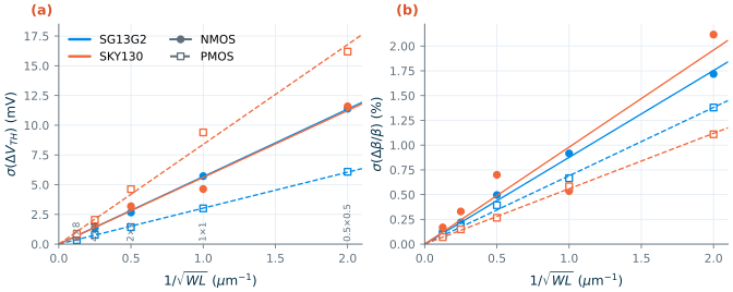
Table 13.3. Pelgrom constants extracted from the PDK mismatch models (strong inversion, tt, 27 °C).
| Constant | SG13G2 NMOS | SG13G2 PMOS | SKY130 NMOS | SKY130 PMOS |
|---|---|---|---|---|
| \(A_{VT}\) (mV·µm) | 5.7 | 3.0 | 5.6 | 8.4 |
| \(A_\beta\) (%·µm) | 0.88 | 0.69 | 0.98 | 0.56 |
| Area for \(\sigma(\Delta V_{TH})\) = 1 mV | 32 µm² | 9.2 µm² | 31 µm² | 70 µm² |
The SG13G2 values match the model parameters: \(\sqrt{2}\times 3.9 = 5.5\) mV·µm for the NMOS and \(\sqrt{2}\times 2.2 = 3.1\) mV·µm for the PMOS. Surveys of many processes find \(A_{VT}\) shrinking roughly in proportion to the oxide thickness from one technology generation to the next [76]. Between these two processes the rule does not hold: the SG13G2 NMOS, with half the oxide thickness of the SKY130 NMOS, matches no better. The SKY130 PMOS has the largest threshold mismatch of the four, almost three times that of the SG13G2 PMOS: a matched PMOS current mirror needs about eight times more area in SKY130.
The demo below rolls the dice for you: pick a PDK, a device and a gate area, draw pairs one by one, and watch their threshold differences pile up into the Gaussian of Eq. (13.11), beside the Monte Carlo points of Figure 13.8.
13.7 Offset
The offset of a differential pair
The input offset voltage \(V_{OS}\) of a differential pair is the differential input that makes the two drain currents equal. Setting \(\Delta I_D = 0\) in Eq. (13.12) and adding the two uncorrelated terms:
Key equation · Offset of a differential pair
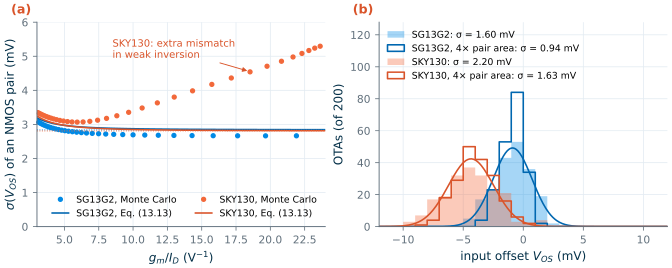
\[\sigma^2(V_{OS}) = \sigma^2(\Delta V_{TH}) + \left(\frac{\sigma(\Delta\beta/\beta)}{g_m/I_D}\right)^2 = \frac{1}{WL}\left[A_{VT}^2 + \left(\frac{A_\beta}{g_m/I_D}\right)^2\right]. \tag{13.13}\]At high gm/ID (weak and moderate inversion) only the threshold term remains; at low gm/ID the current-factor term adds to it.
Figure 13.9a tests Eq. (13.13) on the 2 × 2 µm NMOS pairs, using the offset of every pair at every point of the sweep. In SG13G2 the Monte Carlo result follows the equation within 7 % over the whole range: 2.82 mV at \(g_m/I_D\) = 5 and 2.67 mV at 15. In SKY130 it does only in strong inversion. Above \(g_m/I_D \approx 8\) the offset rises, to 4.07 mV at 15 and 4.74 mV at 20, 44 % and 68 % above Eq. (13.13), because the SKY130 models add a separate random term to the subthreshold parameter voff, which only matters in weak and moderate inversion. Pelgrom’s two constants do not describe that; read the offset at your gm/ID from a Monte Carlo run instead.
The offset of the OTA
In the 5T OTA a mismatch of the mirror \(M_3\)–\(M_4\) also unbalances the currents. A mirror error \(\Delta I/I\) is cancelled by an input voltage \(\Delta I/g_{m1}\), so the mirror’s own \(\Delta V_{GS}\) reaches the input multiplied by \(g_{m3}/g_{m1}\):
\[\sigma^2(V_{OS}) = \sigma^2(V_{OS,12}) + \left(\frac{g_{m3}}{g_{m1}}\right)^2\sigma^2(V_{OS,34}), \tag{13.14}\]with each pair term from Eq. (13.13) at that pair’s own size and gm/ID [51, 76].
Worked example 13.2 · Offset of Chapter 10’s 5T OTA, by hand and by Monte Carlo
SG13G2. The input pair (13.68 × 1 µm = 13.68 µm², \(g_m/I_D\) = 16) gives \(\sqrt{5.7^2 + (0.88/16\cdot 10)^2}\big/\sqrt{13.68}\) = 1.54 mV. (The factor 10 converts %·µm into mV·µm per V⁻¹.) The mirror (14.85 µm², \(g_m/I_D\) = 10) gives 0.81 mV, times \(g_{m3}/g_{m1} = 10/16 = 0.63\): 0.50 mV. Eq. (13.14): \(\sigma(V_{OS}) = \sqrt{1.54^2 + 0.50^2}\) = 1.62 mV.
SKY130. Pair (16.41 µm²): 1.39 mV; mirror (17.28 µm²): 2.02 mV × 0.63 = 1.26 mV; in total 1.88 mV. The SKY130 PMOS mismatch makes the mirror almost as important as the pair.
Monte Carlo. Two hundred copies of each OTA, each with its own random devices and its own 10 µA reference, sit in one netlist, each connected as a unity-gain buffer with the input at Chapter 10’s common-mode level; one operating-point run gives all 200 offsets (Figure 13.9b). The standard deviation is 1.60 mV in SG13G2, 1 % below the hand value, and 2.20 mV in SKY130, 17 % above it. The SKY130 error is the moderate-inversion effect of Figure 13.9a: reading the pair term from the Monte Carlo curve at \(g_m/I_D\) = 16 instead of Eq. (13.13) gives 2.54 mV, now 15 % high. With 200 samples the simulated σ itself is uncertain by about ±5 % (one standard deviation).
Systematic offset. The distributions are not centred on zero: the mean offset is −0.9 mV in SG13G2 and −4.4 mV in SKY130, close to a run without mismatch (−1.1 and −4.3 mV). It comes from the 5T OTA’s structure: the drain of \(M_1\) sits at \(V_{DD} - V_{SG3}\) while the drain of \(M_2\) sits at the output, so the two halves can have different \(V_{DS}\) and, with finite output resistance, different currents. Chapter 10 chose the SG13G2 common-mode level (0.7 V) close to the mirror node (0.68 V), so the offset is small there; in SKY130 the output at 1.1 V sits 0.47 V above the mirror node. It is deterministic, so it can be designed out (Chapter 12 discusses the two-stage version).
With the input pair four times larger, the random offset falls to 0.94 mV in SG13G2, a factor of 1.7 rather than 2, because the mirror’s 0.5 mV did not change; Eq. (13.14) predicts 0.92 mV. In SKY130 it falls only to 1.63 mV, a factor of 1.35, because there the mirror’s 1.3–1.5 mV is now the larger term. The two-stage OTA of Chapter 12, with its larger input pair, has a random offset of 1.33 mV in SG13G2 and 4.08 mV in SKY130 (200 copies each, means −0.2 and −0.5 mV); in SKY130 its short PMOS mirror (10 × 0.5 µm) dominates.
Designing for low offset
- Area. Offset falls as \(1/\sqrt{WL}\): four times the area for half the offset. Every square micrometre adds gate capacitance, \(C_{ox}WL\), so for a given threshold mismatch the product \(\sigma^2(\Delta V_{TH})\cdot C_{gate} = A_{VT}^2 C_{ox}\) is fixed by the process. Kinget showed that this ties precision to speed and power: each halving of the offset costs four times the power at the same speed [76]. Trimming, auto-zeroing or chopping are cheaper beyond a point.
- gm/ID. Bias the input pair at high gm/ID, where the \(A_\beta\) term of Eq. (13.13) vanishes (but check the SKY130 weak-inversion penalty), and the mirror at low gm/ID, which shrinks \(g_{m3}/g_{m1}\) in Eq. (13.14). These are the same choices that lower the noise in Section 13.4.
- Layout. Eq. (13.11) holds only for devices that see the same surroundings. Gradients of oxide thickness, temperature and stress across the die add a systematic mismatch that grows with the distance between the devices. Common-centroid and interdigitated layouts, dummy devices and identical orientation remove it (Chapter 15).
What this means for your design
For Chapter 10’s 20 MHz OTA, the input pairs of 14–16 µm² give a 3σ offset of about 5 mV (SG13G2) and 7 mV (SKY130). For σ(VOS) = 1 mV, Eq. (13.13) says each input device needs about 33 µm² in SG13G2 and about 70 µm² in SKY130 (using the Monte Carlo value of 8.4 mV·µm at gm/ID = 16), and a 3σ offset of 1 mV needs nine times that. In SKY130 the PMOS mirror must grow with it, because its mismatch is already as large as the pair’s. The gate capacitance then sets the bandwidth of whatever drives the OTA. Decide early whether area, calibration or chopping is the cheaper route.
13.8 Monte Carlo in ngspice
A Monte Carlo simulation repeats a circuit many times with random device parameters drawn from the PDK’s statistical models, and reports the distribution of the result. ngspice evaluates the random functions (agauss, gauss) in the model files when it reads the netlist, separately for every subcircuit instance. Two consequences make Monte Carlo fast and simple:
- Many copies in one netlist. A netlist with 200 copies of the OTA gives 200 independent samples from one operating-point run. In SKY130, where the full model library takes about 20 s to load, this is far faster than 200 separate runs; the 1600-transistor sweep of Section 13.6 is a single run.
- Reproducibility. The option
seedfixes the random sequence, so a result can be repeated exactly. Without it every run draws new numbers.
* Monte Carlo of mismatch: identical NMOS pairs in one netlist (repeat the instance lines as needed)
.lib cornerMOSlv.lib mos_tt_mismatch
.options seed=1301
Vd d 0 0.6
Vg g 0 0
* mm_ok=1 switches the mismatch on for this instance (the subcircuit default is 0)
XMA0 d g 0 0 sg13_lv_nmos W=2u L=2u ng=1 m=1 mm_ok=1
XMB0 d g 0 0 sg13_lv_nmos W=2u L=2u ng=1 m=1 mm_ok=1
.save @n.xma0.nsg13_lv_nmos[ids] @n.xmb0.nsg13_lv_nmos[ids]
.control
dc Vg 0.1 1.2 0.02
wrdata pairs.txt @n.xma0.nsg13_lv_nmos[ids] @n.xmb0.nsg13_lv_nmos[ids]
.endc
.end
* Monte Carlo of mismatch: identical NMOS pairs in one netlist (repeat the instance lines as needed)
* tt_mm = typical models with device mismatch; mc = mismatch plus global process variation
.lib "$PDK_ROOT/sky130A/libs.tech/ngspice/sky130.lib.spice" tt_mm
.options seed=1302
Vd d 0 0.9
Vg g 0 0
XMA0 d g 0 0 sky130_fd_pr__nfet_01v8 W=2 L=2 nf=1 mult=1 m=1
XMB0 d g 0 0 sky130_fd_pr__nfet_01v8 W=2 L=2 nf=1 mult=1 m=1
.save @m.xma0.msky130_fd_pr__nfet_01v8[id] @m.xmb0.msky130_fd_pr__nfet_01v8[id]
.control
dc Vg 0.1 1.8 0.02
wrdata pairs.txt @m.xma0.msky130_fd_pr__nfet_01v8[id] @m.xmb0.msky130_fd_pr__nfet_01v8[id]
.endc
.end
Our scripts generate these netlists with Python loops: tools/figs/ch13_mismatch.py for the pairs and the OTAs. When a circuit is too large to copy hundreds of times, run it in a loop instead: ngspice’s mc_source command reloads the netlist and draws new random numbers on each pass [36].
Common pitfall · A Monte Carlo run with no mismatch in it
Mismatch is off unless you switch it on, and the switch is different in each PDK. In SG13G2 you need both the
mos_tt_mismatchlibrary section andmm_ok=1on each instance; the Xschem symbols setmm_ok=1by default, but a hand-written netlist that copies onlyW,Landnggets the subcircuit default, 0, and every “random” device is identical. In SKY130 the plainttsection has no mismatch; usett_mm(mismatch only) ormc(mismatch and process). Always check that a Monte Carlo run has a spread: run two identical devices and compare their currents.
How many samples are enough? The standard deviation estimated from \(N\) samples has a relative uncertainty of about \(1/\sqrt{2N}\): 200 samples give σ to ±5 %, 1000 samples to ±2 %. Yield estimates far in the tails (a 4σ or 6σ specification) need far more samples or a different method.
Try it · Lab 7
Lab 7 runs the noise analysis of your OTA from Lab 5 or 6, compares it with Eq. (13.8), and then runs a Monte Carlo of its offset with 200 copies in one netlist. Change the input-pair area and gm/ID and watch both the noise and the offset histogram move.
- Thermal noise is white, \(4kT\gamma/g_m\) at the gate: only more \(g_m\), which costs current, lowers it. Flicker noise is \(K_f'/(WLf)\): only more gate area lowers it, and its corner falls as \(1/L^2\).
- The PDK models give very different noise constants: SG13G2 NMOS \(\gamma \approx 0.8\) with the PMOS 2.7× noisier in flicker; SKY130 NMOS \(\gamma \approx 2\) with 4.7× the PMOS flicker. Choose the input device from these numbers.
- Refer noise to the input. In the 5T OTA the load adds noise in proportion to \(g_{m3}/g_{m1}\), so bias loads at low gm/ID. Hand formulas with two constants per device were within 1–3 % of ngspice.
- kT/C noise depends only on the capacitance: 64 µV rms on 1 pF at 27 °C. A closed-loop amplifier’s integrated noise has the same form, \(kT/C_L\) times a factor.
- Mismatch follows Pelgrom’s law, \(A/\sqrt{WL}\). Extracted constants: \(A_{VT}\) = 5.7/3.0 mV·µm (SG13G2 N/P) and 5.6/8.4 mV·µm (SKY130 N/P). SKY130 adds extra mismatch in weak inversion.
- Chapter 10’s 5T OTA has a random offset of 1.6 mV (SG13G2) and 2.2 mV (SKY130) rms by Monte Carlo, within 1 % and 17 % of the hand prediction; 4× input-pair area lowered it to 0.9 and 1.6 mV, limited by the mirror. Monte Carlo with many copies in one netlist is fast; switch the mismatch models on explicitly.
Further reading
- B. Razavi, Design of Analog CMOS Integrated Circuits [51], chapter 7: the clearest textbook treatment of noise in amplifiers, with the input-referred approach used here.
- M. J. M. Pelgrom, A. C. J. Duinmaijer and A. P. G. Welbers [75]: the original matching paper.
- P. R. Kinget [76]: how mismatch ties together area, power, speed and accuracy, with design examples.
- W. Sansen, Analog Design Essentials [62]: noise and offset of every common circuit, and the dynamic offset-cancellation techniques (chopping, auto-zero) that this chapter only mentions.
- C. C. Enz and E. A. Vittoz [59]: thermal and flicker noise across all inversion levels in the EKV framework.