Chapter 24
Reliability: Electromigration, Latch-up and Antennas
A circuit that simulates perfectly can still fail in the field: wires wear out under current, parasitic thyristors latch, and plasma charge breaks gate oxides during manufacture. Layout is where each of these is prevented. This chapter puts numbers on every mechanism from the documents and decks of SG13G2 and SKY130, simulates the parasitic thyristor, and draws the layouts that the latch-up and antenna checks reject and accept.
- State the voltage limits of the thin and thick gate oxides and of the junctions of both PDKs, and explain what happens beyond them.
- Derive Black’s equation, read the electromigration limits of both PDKs, and size wires and vias for a given current and temperature.
- Estimate the temperature rise of a wire and of a device from its thermal resistance, and say when heating, not electromigration, limits the current.
- Explain latch-up with the parasitic thyristor of a CMOS inverter, predict its trigger and holding currents, and prevent it with taps and guard rings that pass the latch-up rules.
- Calculate antenna ratios by hand, check them with the decks of both PDKs, and fix violations with jumpers and diodes.
Contents
Chapter 23 explained the geometric rules, the ones that make a layout manufacturable. This chapter is about the rules that make it last. They are of a different kind: most of them are not about the shape of a polygon but about what flows through it (current, heat, charge) and about what parasitic devices the polygons form together. Several of them are not checked by the default DRC run at all, and one (the current-density limit) is checked by no deck of either PDK. Everything here is computed from the PDK documents and decks or simulated, in IIC-OSIC-TOOLS [35]; Hastings’s chapter on failure mechanisms is the best general treatment [61].
python3 tools/layout/ch24/rel_layouts.py     # latch-up and antenna layouts, DRC + antenna checks, 3D models (47 s)
python3 tools/figs/ch24_reliability.py       # the figures and tools/figs/ch24_reliability_numbers.json
24.1 Electrical overstress and safe operating limits
Electrical overstress (EOS) is any voltage or current beyond what a structure is built to take. It ranges from the instantaneous (a gate oxide that breaks down, a junction driven into avalanche, a wire that melts) to the slow (an oxide or a transistor that degrades over years at a voltage only slightly too high). Electrostatic discharge is a special case, short and very large, and gets its own chapter (Chapter 29). Every PDK states the limits within which its devices are qualified, and Table 24.1 collects them.
Table 24.1. Voltage limits of the devices of both PDKs [15, 18].
| Quantity | SG13G2 | SKY130 |
|---|---|---|
| Core MOSFET, nominal supply | 1.2 V | 1.8 V |
| Core MOSFET, gate voltage limit | \(V_{GS}\) ≤ 1.65 V at 125 °C | \(V_{GS}\), \(V_{DS}\) ≤ 1.95 V (model validity) |
| Core gate oxide | 2.65 nm (NMOS), 2.45 nm (PMOS) | 4.15 nm (model toxe) |
| Core drain-source breakdown | 2.0 to 2.9 V (\(BV_{DSS}\), \(L\) = 0.13 µm) | not published |
| Thick-oxide MOSFET | 3.3 V: \(V_{GS}\) ≤ 3.3 V, \(L\) ≥ 0.5–0.6 µm | 5 V gate, 10.5 V drain: \(V_{GS}\) ≤ 5.5 V, \(V_{DS}\) ≤ 11 V (g5v0d10v5) |
| Thick gate oxide | 7.5 nm (NMOS), 7.3 nm (PMOS) | not published |
| Thick-oxide drain-source breakdown | 5.3 to 6.3 V | — |
| Junction breakdown (diffusion to well) | 12 V (n+/p-well and p+/n-well) | 10.5 to 12.7 V, by diode type (nominal) |
| MIM capacitor | breakdown ≥ 15 V | models valid to 5 V |
Three things in the table matter for layout.
The oxide sets the hard limit, not the junction. The junctions of both PDKs break down near 12 V, ten times the core supply; the gate oxide of a core transistor is qualified for less than 2 V. At 1.65 V across 2.65 nm the SG13G2 core oxide carries a field of 6.2 MV/cm; at 1.95 V across 4.15 nm the SKY130 one carries 4.7 MV/cm. Dielectric breakdown of silicon dioxide begins around 10 MV/cm, and long before that the oxide wears out slowly (Section 24.7). A core gate must never see a 3.3 V net: not directly, not through a capacitor that couples a 3.3 V edge, and not through a pass device that lets an I/O voltage through. Level shifters and the thick-oxide devices exist for exactly this.
The limits come with a temperature. SG13G2 qualifies its core devices at 1.65 V at 125 °C, its electromigration limits at 105 °C (Section 24.2). A limit without its temperature is half a number.
The thick-oxide devices need longer gates. SG13G2’s 3.3 V devices are specified for gate lengths of at least 0.5 µm (PMOS) and 0.6 µm (NMOS), and its layout rules widen every well spacing around them (Table 23.4): the higher voltage needs longer channels against punch-through and wider junction spacings against breakdown.
SG13G2 vs SKY130 · Where the limits are written
IHP publishes a process specification with pass/fail limits for every device and the conditions under which they hold, including the 125 °C gate-voltage limit and the electromigration rules [15]. SkyWater’s open documentation gives the voltage range over which each SPICE model is valid and a table of diode breakdown voltages [18], but no lifetime-qualified limits. In SKY130 treat the model-validity range as the absolute maximum, not as a recommended operating range.
24.2 Electromigration and current-density rules
A current in a metal is a stream of electrons, and the electrons collide with the metal atoms. Each collision passes on a little momentum, so the current pushes the atoms, very slowly, in the direction of the electron flow. This is electromigration (EM). Where the atomic flux leaving a region exceeds the flux arriving, for example at a via that blocks the flow or at a junction of grain boundaries, the metal thins and a void grows until the line opens; where atoms pile up, a hillock grows until it shorts to a neighbour [123, 68].
Black’s equation
The force of the “electron wind” on a metal ion is proportional to the current density \(j\): \(F = Z^* e \rho j\), where \(\rho\) is the resistivity and \(Z^*\) an effective charge number. An atom that can jump to a neighbouring site with diffusivity \(D = D_0 e^{-E_a/kT}\) drifts under this force with the velocity \(v = DF/kT\) (the Nernst–Einstein relation), so the atomic flux, \(N\) atoms per unit volume times \(v\), is
\[J_a = \frac{N D_0 Z^* e \rho}{kT}\, j\, e^{-E_a/kT}. \tag{24.1}\]A line fails when a fixed volume of metal has been carried away from a site of flux divergence. The time to do so is inversely proportional to the flux, \(t_f \propto kT\,e^{E_a/kT}/j\). Measured lifetimes follow this form with a stronger current dependence, because a void must first nucleate (the wind builds up mechanical stress until it does) before it grows. Black summarized the measurements in the empirical law that still defines every EM rule [123]:
Key equation · Black’s equation for the median time to failure
\[\mathrm{MTTF} = A\, j^{-n}\, e^{E_a/kT}, \tag{24.2}\]with \(n \approx 2\) when void nucleation dominates and \(n \approx 1\) when growth dominates, and \(E_a\) of about 0.7 to 0.9 eV for aluminium lines with a little copper added, the usual metallization of aluminium processes [68, 61].
A foundry measures MTTF on test lines at high current and temperature, and then uses Eq. (24.2) to find the current density at which a stated fraction of lines survives a stated lifetime at a stated temperature. For two operating points with the same lifetime, Eq. (24.2) gives the temperature derating
\[\frac{j_{max}(T)}{j_{max}(T_{ref})} = \exp\!\left[\frac{E_a}{n k}\left(\frac{1}{T} - \frac{1}{T_{ref}}\right)\right]. \tag{24.3}\]Derivation · From the lifetime to the derating, and what a doubling of current costs
Write Eq. (24.2) at the reference point and at the new point and require the same MTTF: \(j^{-n} e^{E_a/kT} = j_{ref}^{-n} e^{E_a/kT_{ref}}\). Take the logarithm, \(-n\ln j + E_a/kT = -n\ln j_{ref} + E_a/kT_{ref}\), and solve for \(\ln(j/j_{ref})\): Eq. (24.3). With \(E_a\) = 0.8 eV and \(n\) = 2, \(E_a/nk\) = 4640 K. From 105 °C (378 K) to 125 °C (398 K), \(1/T - 1/T_{ref}\) = −1.33 × 10⁻⁴ K⁻¹, so the allowed current density falls by \(e^{-0.62}\) = 0.54.
At fixed temperature, the lifetime scales as \(j^{-n}\): with \(n\) = 2 a line run at twice its rated current lasts a quarter as long. Because the rule is a statistical statement (a failure fraction, not a sharp threshold), a design that exceeds it by 10 % does not fail at once; it fails earlier, and more often, than the qualification promised.
Two refinements explain details of the rules. Short lines are immune: the atoms swept to the downstream end of a short line build up a compressive stress whose gradient pushes back against the wind, and below a critical product of current density and length the two balance and no void forms (the Blech length) [124]. And narrow lines last longer: when a line is narrower than the metal grains, the grain boundaries cross it like the joints of a bamboo stem and the fast diffusion path along them is interrupted [61]. A current that reverses direction (a true AC current) largely undoes its own damage; there, the limit becomes heating (Section 24.3).
The limits of both PDKs
SG13G2 publishes its limits in section 2.15 of the process specification, for less than 0.01 % failures in 11 years of operation at 105 °C [15]. They are given per micrometre of line width, and per contact or via (Table 24.2). No DRC deck checks them; the designer does, from the currents in the schematic.
SKY130 has no published limits. SkyWater’s periphery rules list electromigration as rule x.4, “electrical design rules cover layout guidelines for electromigration”, flagged as not checkable, with no value [18]; neither the open PDK nor its decks contain a current-density table. For the examples of this chapter we therefore use an estimate: the SG13G2 Metal1 limit expressed per unit cross-section (1 mA/µm ÷ 0.42 µm = 2.38 mA/µm², i.e. 0.24 MA/cm²) applied to the SKY130 metal thicknesses, and the SG13G2 Via1 limit per unit cut area (0.4 mA ÷ 0.19² µm² = 11.1 mA/µm²) applied to the SKY130 cut sizes. Both processes use etched aluminium wiring with tungsten plugs (Chapter 17), so the estimate should have the right order of magnitude, but it is ours, not the foundry’s: for a tape-out, ask your shuttle provider for the qualified numbers.
Table 24.2. DC current limits of the metals and cuts. SG13G2: process specification, 11 years at 105 °C [15]. SKY130: our estimate, scaled from SG13G2 by cross-section and cut area (thicknesses and cut sizes from Magic's sky130A.tech [20]).
| Layer (thickness) | SG13G2 | Layer (thickness) | SKY130, estimate |
|---|---|---|---|
| Metal1 (0.42 µm) | 0.36 mA for \(w\) = 0.16–0.36 µm; 1 mA/µm above | li1 (0.10 µm, TiN) | none: limited by its 12.8 Ω/□ |
| Metal2–Metal5 (0.49 µm) | 0.6 mA for \(w\) = 0.20–0.30 µm; 2 mA/µm above | met1, met2 (0.36 µm) | 0.86 mA/µm (0.12 mA at 0.14 µm) |
| TopMetal1 (2.0 µm) | 15 mA/µm (24.6 mA at 1.64 µm) | met3, met4 (0.845 µm) | 2.0 mA/µm (0.60 mA at 0.30 µm) |
| TopMetal2 (3.0 µm) | 16 mA/µm (32 mA at 2.0 µm) | met5 (1.26 µm) | 3.0 mA/µm (4.8 mA at 1.6 µm) |
| Cont (0.16 µm) | 0.3 mA per contact | licon, mcon (0.17 µm) | 0.32 mA per cut |
| Via1–Via4 (0.19 µm) | 0.4 mA per via | via (0.15 µm); via2, via3 (0.20 µm) | 0.25 mA; 0.44 mA |
| TopVia1 (0.42 µm); TopVia2 (0.90 µm) | 1.4 mA; 10 mA | via4 (0.80 µm) | 7.1 mA |
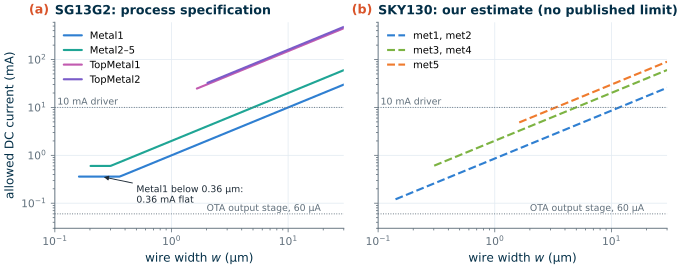
Figure 24.1 shows the limits against width. Two features stand out. The thin metals of SG13G2 start flat: a Metal1 line between 0.16 and 0.36 µm wide may carry 0.36 mA whatever its width, which at the minimum width is 5.4 mA/µm² of cross-section, against 2.4 mA/µm² for a wide line. And the two thick top metals carry ten times more per micrometre of width than the thin ones, because they are four to six times thicker and have larger grains: they are where supply rails and high-current routes belong.
Worked example 24.1 · Sizing the supply wires and vias of the course OTA’s output stage
The output stage of the two-stage OTA of Chapter 12 carries \(I_7\) = 60 µA from \(V_{DD}\) through M6 and M7 to ground, in both PDKs; the whole OTA draws 90 µA (
tools/figs/ch12_numbers.json). Size the wires and cuts that bring this current to the sources of M6 and M7, for operation at 125 °C.Derating. Eq. (24.3) with \(E_a\) = 0.8 eV, \(n\) = 2: the limits of Table 24.2 shrink to 0.54 of their value at 125 °C (0.50 to 0.58 for \(E_a\) = 0.9 to 0.7 eV).
SG13G2. A minimum-width Metal1 line (0.16 µm) carries 0.36 mA × 0.54 = 0.19 mA at 125 °C, 3.2 times the 60 µA. One Via1 carries 0.4 × 0.54 = 0.22 mA, 3.6 times. The OTA’s supply spines are 0.5 µm wide Metal3 (Chapter 15): 2 mA/µm × 0.5 µm × 0.54 = 0.54 mA, six times the full 90 µA.
SKY130 (estimate). A minimum met1 line (0.14 µm) carries 0.86 mA/µm × 0.14 µm × 0.54 = 65 µA: only 8 % above 60 µA. Widen it to 0.3 µm (0.14 mA, 2.3 times). One mcon or via is ample (0.32 and 0.25 mA × 0.54). li1 has no EM limit of its own, but 10 µm of minimum li1 is 12.8 Ω/□ × 10/0.17 = 750 Ω, 45 mV at 60 µA: in SKY130 the resistance of li1, not its lifetime, keeps it to short stubs over the contacts.
The same stage at 10 mA, as an output driver might need: at 125 °C SG13G2 Metal2 must be 10 mA / (2 mA/µm × 0.54) = 9.3 µm wide with 10 / (0.4 × 0.54) = 47 Via1 cuts, or a single TopMetal1 line at its minimum width of 1.64 µm (13 mA at 125 °C). The SKY130 estimate asks for 9.2 µm of met3 and 75 vias of 0.15 µm.
What decides. For the bias currents of an analog block, EM is satisfied by the minimum width in SG13G2 and almost so in SKY130; IR drop, redundancy (two cuts instead of one, in case one is poorly formed) and matching decide the wire widths. EM decides only for milliampere currents: output drivers, supply rails of large blocks, bias distribution trunks, and the pads.
Common pitfall · Checking the average current of a supply rail
A rail that feeds a switching block (a comparator, a clocked bias, a digital section) carries spikes many times its average. Electromigration responds to the average current of a unidirectional flow (with some relief for short pulses), heating responds to the RMS current, and fusing to the peak. Size for all three: the average from the EM rule, the RMS from Section 24.3, and check the peak against the current a short pulse can melt (Chapter 29).
24.3 Self-heating of wires and devices
Every wire dissipates \(I^2R\), and the heat has to cross the oxide to the silicon, which is a good heat sink: silicon conducts heat a hundred times better than silicon dioxide (148 against about 1.4 W/(m·K)). A wire of width \(w\) at height \(h\) above the silicon therefore sits on a thermal resistance set almost entirely by the oxide beneath it. If the heat spreads at 45° on both sides, the path at depth \(z\) is \(w + 2z\) wide, and the thermal resistance per unit length is
\[\theta' = \int_0^h \frac{dz}{k_{ox}(w+2z)} = \frac{\ln(1 + 2h/w)}{2k_{ox}}. \tag{24.4}\]The wire dissipates \(P' = I^2 R_\square / w\) per unit length, so its temperature rise is
Key equation · Temperature rise of a long wire
\[\Delta T = \frac{I^2 R_\square}{w}\cdot\frac{\ln(1+2h/w)}{2k_{ox}}. \tag{24.5}\]
For a wide wire (\(w \gg h\)) the logarithm becomes \(2h/w\) and \(\Delta T = j^2 \rho\, t\, h / k_{ox}\): the temperature rise grows with the square of the current density, with the thickness \(t\) and with the height \(h\). That is bad news for the thick top metals, which carry the highest current densities, are the thickest, and sit highest: SG13G2’s TopMetal2 is 10.8 µm above the silicon.
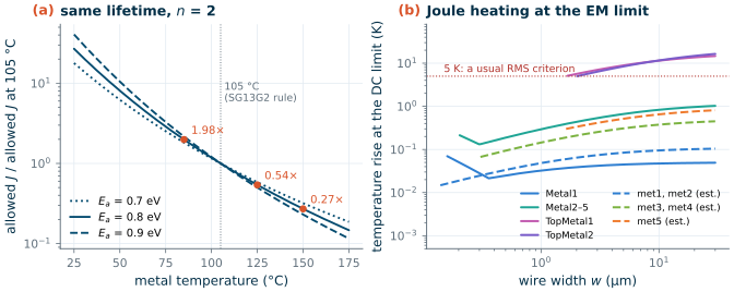
tools/3d/stacks.py (for grouped layers, the highest).Figure 24.2b applies Eq. (24.5) to every metal at its DC limit. The thin metals hardly notice their own current: SG13G2 Metal1 rises by 0.03 K at 1 µm width, Metal5 by 0.8 K at 10 µm. The top metals rise by 11 to 12 K at 10 µm, and that heat raises the temperature in Eq. (24.3) and so lowers the very limit the wire is running at. Foundries therefore give a second, RMS limit, usually for a temperature rise of a few kelvin. With a 5 K criterion, Eq. (24.5) gives 105 mA for a 10 µm TopMetal2 line, below its 160 mA DC limit, but 12 mA for a 1 µm Metal1 line, twelve times its DC limit. The two limits apply to different currents: the DC (EM) limit to the average of a unidirectional current, the RMS (heating) limit to any current. A clock or RF line whose current reverses can run far above the DC limit of a thin metal; a top-metal supply rail is limited by heating first.
What this means for your design
For the thin metals, size for electromigration and IR drop; heating follows. For the thick top metals, check the RMS current against heating too, and remember that a hot rail derates itself. The SKY130 top metal (met5, 1.26 µm, 5 µm above the silicon) heats less than SG13G2’s TopMetal2 at the same current per micrometre, but it is also allowed less current.
Devices
A transistor dissipates \(I_D V_{DS}\) in its channel. Its heat spreads into the silicon below, and a source of area \(A\) on a large block of silicon sees a spreading resistance of about \(R_{th} = 1/(4 k_{Si} a)\), with \(a = \sqrt{A/\pi}\) the radius of a disc of the same area. The output transistor M6 of the course OTA is 24 fingers of 3.33 µm in SG13G2, about 70 µm² of active area: \(R_{th}\) ≈ 360 K/W, and at 60 µA and 0.6 V it heats by 0.013 K. In SKY130 (12 fingers of 5 µm, about 47 µm², 0.9 V) it is 0.024 K. Self-heating is irrelevant for the course OTA.
It is not irrelevant for small, high-current devices. The SG13G2 HBT model carries its own thermal network: rth = 3.26 kK/W × (4/Nx)0.9 for npn13G2, so a single-emitter device has 11.4 kK/W [14]. At 1 mA and 1.2 V it runs 14 K above the substrate, with a thermal time constant rth·cth of about 5 ns: fast enough that its temperature follows the signal and modulates its \(V_{BE}\), which is why the model includes it. The same physics sets the current limits of the SG13G2 poly resistors: 1.2 mA per µm of width for rppd and 0.6 mA/µm for rhigh (11 years at 105 °C), while rsil is limited by its contacts [15].
24.4 Latch-up: the parasitic thyristor
Every CMOS inverter contains a four-layer p-n-p-n structure: the p+ source of the PMOS, the n-well, the p-substrate and the n+ source of the NMOS. The four layers form two bipolar transistors, a vertical PNP (emitter: p+ source; base: n-well; collector: substrate) and a lateral NPN (emitter: n+ source; base: substrate; collector: n-well), and each one’s collector feeds the other’s base. That is a thyristor, or silicon-controlled rectifier (SCR) [61, 55]. As long as both transistors are off, it does nothing. If something turns one of them on, the loop can regenerate, and the thyristor latches into a low-resistance path from \(V_{DD}\) to ground that stays on until the supply is removed: latch-up. The current is limited only by the supply and the wiring, and it can destroy the metal, the contacts or the junctions within milliseconds.
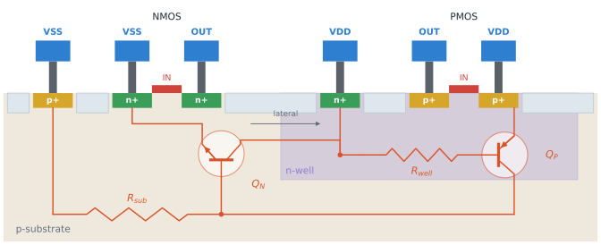
tools/3d/stacks.py (contacts 0.64 µm, Metal1 0.42 µm); widths, well and junction depths schematic. Rwell and Rsub are the resistances from the bases of the two transistors to their ties; the n-well tie is placed between the two transistors, where a guard ring would put it.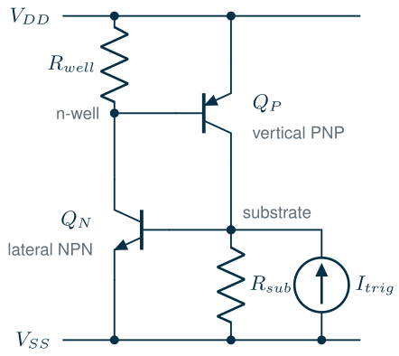
When does it latch?
Figure 24.4 shows the circuit. The two resistors are the key: each shunts the base-emitter junction of one transistor, so a transistor turns on only when the current through its resistor develops about one \(V_{BE}\), some 0.7 V. The conditions follow by walking once around the loop.
Derivation · The holding condition of the thyristor with its shunt resistors
Assume both transistors conduct, with \(V_{BE}\) ≈ \(V_{EB}\) ≈ \(V_{on}\). Let QN carry a collector current \(I_{CN}\), drawn from the n-well node. Of this current, \(V_{on}/R_{well}\) flows through \(R_{well}\) (which has \(V_{EB}\) of QP across it), and the rest is QP’s base current: \(I_{BP} = I_{CN} - V_{on}/R_{well}\). QP delivers \(\beta_p I_{BP}\) into the substrate node, of which \(V_{on}/R_{sub}\) leaves through \(R_{sub}\), and the rest is QN’s base current. QN then returns
\[I_{CN}' = \beta_n\left[\beta_p\left(I_{CN} - \frac{V_{on}}{R_{well}}\right) - \frac{V_{on}}{R_{sub}}\right].\]The loop sustains itself if \(I_{CN}' \geq I_{CN}\), which requires
\[\beta_n \beta_p > 1 \quad\text{and}\quad I_{CN} \geq \frac{\beta_n V_{on}\left(\beta_p/R_{well} + 1/R_{sub}\right)}{\beta_n\beta_p - 1}. \tag{24.6}\]The first condition is the textbook one; the second says that with shunt resistors the loop gain exceeds one only above a minimum current, the holding current. Small resistances raise it in proportion. Below it the thyristor turns itself off.
Three conditions must hold at once for latch-up [61]:
- Loop gain. \(\beta_n\beta_p > 1\). The PNP is a real device of both PDKs, the substrate PNP used in bandgap references, and its model gives \(\beta_F\) = 1.1 in SG13G2 and 16.6 in SKY130 (Chapter 14). The lateral NPN has no model; its gain depends on the distance from the n+ source to the n-well, and we assume \(\beta_n\) = 10. Either way the product exceeds one in both PDKs.
- A trigger. Something must drive one base-emitter junction into conduction: a current \(I_{trig}\) ≈ \(V_{on}/R_{sub}\) injected into the substrate, or \(V_{on}/R_{well}\) drawn from the well. Typical triggers are an I/O pin pulled below ground or above the supply (forward-biasing a drain junction), a fast supply ramp that charges the well capacitance, or the breakdown of a junction.
- Holding. The supply must deliver more than the holding current of Eq. (24.6) at a voltage above the holding voltage \(V_H\), about \(V_{on}\) plus a saturated \(V_{CE}\) plus the ohmic drops.
Simulating the thyristor
tools/figs/_ch24_scr.py builds the circuit of Figure 24.4 in ngspice for a 10 µm wide inverter. The PNP takes the saturation current density and \(\beta_F\) of each PDK’s substrate PNP model; the NPN has \(I_S\) = 10 aA and \(\beta_F\) = 10; a diode with the junction breakdown voltage of Table 24.1 (12 V in SG13G2, 11.7 V in SKY130) closes the loop when the anode is forced high. The resistances are sheet resistance times squares, from the PDK files: SKY130 n-well 0.95 kΩ/□ and p-well 4.4 kΩ/□ from the extraction section of Magic’s sky130A.tech [20]; SG13G2 p-well 3 kΩ/□ from the layout rules (note 4 of section 6.5) [16]. IHP publishes no n-well sheet resistance (Magic’s IHP technology file marks it “TBD”), so we take 1 kΩ/□, close to SKY130’s. Two layouts are compared:
- Ties at the latch-up limit: each transistor’s tie at the largest distance the rules allow, 20 µm in SG13G2 and 15 µm in SKY130 (Section 24.5), so 2 and 1.5 squares of well: \(R_{well}\) = 2.0 kΩ and \(R_{sub}\) = 6.0 kΩ in SG13G2, 1.4 kΩ and 6.6 kΩ in SKY130.
- Guard rings 1 µm from each transistor on both sides: \(R_{well}\) = 50 Ω and \(R_{sub}\) = 150 Ω in SG13G2, 48 Ω and 220 Ω in SKY130.
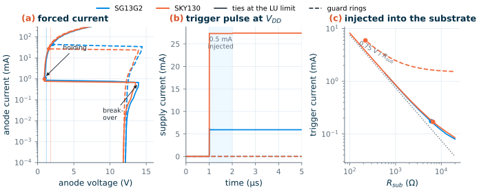
Figure 24.5 shows the result, and Table 24.3 gives the numbers.
Table 24.3. Simulated thyristor of a 10 µm inverter (tools/figs/ch24_reliability_numbers.json).
| Quantity | SG13G2, ties at 20 µm | SG13G2, guard rings | SKY130, ties at 15 µm | SKY130, guard rings |
|---|---|---|---|---|
| \(R_{well}\) / \(R_{sub}\) | 2.0 kΩ / 6.0 kΩ | 50 Ω / 150 Ω | 1.4 kΩ / 6.6 kΩ | 48 Ω / 220 Ω |
| Break-over voltage | 13.9 V | 14.4 V | 13.5 V | 13.9 V |
| Holding voltage / current | 1.02 V / 1.1 mA | 2.07 V / 44 mA | 0.93 V / 0.97 mA | 1.53 V / 27 mA |
| Trigger current at \(V_{DD}\) (substrate injection) | 0.18 mA | does not hold at 1.2 V | 0.17 mA | 6.0 mA |
| Trigger current at 3.3 V | 0.17 mA | 8.2 mA | 0.17 mA | 5.9 mA |
| Supply current after a 0.5 mA pulse | 5.9 mA (latched) | 0 | 27 mA (latched) | 0 |
- The forced-current curve (Figure 24.5a) has the S-shape of every thyristor. The structure blocks until the n-well junction breaks down near 12 V; the breakdown current flows through both resistors, turns both transistors on, and the voltage collapses to the holding point. Only that last part matters on chip: the supplies never reach 12 V, but an injected current can take the thyristor straight to its latched branch.
- The holding voltage of the poorly tied inverter is below both supplies: 1.02 V against 1.2 V in SG13G2, 0.93 V against 1.8 V in SKY130. A low supply is not a protection. Once triggered, the inverter of Figure 24.5b stays latched after the 0.5 mA pulse has ended, and only removing the supply would release it.
- The trigger current is set by \(R_{sub}\), almost exactly \(V_{on}/R_{sub}\) with \(V_{on}\) ≈ 0.75 V (Figure 24.5c): 0.17 mA with the ties at the rule limit. That is a small current: an I/O pin pulled 0.5 V below ground through a few kilohms delivers it.
- Guard rings change everything at once. They raise the trigger current 35-fold in SKY130 (to 6 mA) and the holding current 30 to 40-fold, and in SG13G2 they push the holding voltage (2.07 V) above the 1.2 V core supply, so the core inverter cannot latch at all; on a 3.3 V I/O supply it still can, at 8.2 mA.
Worked example 24.2 · The trigger current, by hand
For the SKY130 inverter with its ties at the 15 µm limit, QN turns on when the injected current develops \(V_{on}\) ≈ 0.75 V across \(R_{sub}\) = 4.4 kΩ/□ × 15/10 = 6.6 kΩ: \(I_{trig}\) ≈ 0.75/6600 = 0.11 mA. The simulation gives 0.17 mA, because part of the injected current is collected by QN’s base only after QP has turned on too. The holding current from Eq. (24.6), with \(\beta_n\) = 10, \(\beta_p\) = 16.6 and \(R_{well}\) = 1.4 kΩ, is \(I_{CN}\) ≥ 10 × 0.75 × (16.6/1425 + 1/6600) / 165 = 0.54 mA of QN collector current; the simulated supply current at the holding point, which also contains QP’s emitter current, is 0.97 mA. With the guard ring (\(R_{well}\) = 48 Ω, \(R_{sub}\) = 220 Ω) the same formulas give 3.4 mA and 16 mA, against 6.0 and 27 mA simulated. The hand formulas get the order of magnitude and, more usefully, the scaling: both currents are inversely proportional to the tie resistances.
The simulation has assumptions you should keep in mind: the NPN gain, the SG13G2 n-well sheet resistance and the series resistances that set the holding voltage are estimates, and a real substrate adds a deep, three-dimensional path that a sheet resistance only approximates. The scaling with the resistances does not depend on them, and that is what layout controls.
24.5 Taps, guard rings and latch-up rules
Layout fights latch-up on all three conditions. Ties (taps) close to every transistor make \(R_{well}\) and \(R_{sub}\) small, which raises the trigger and holding currents (Figure 24.5c). Guard rings, continuous ties around a group of devices, do the same from every side and also collect injected carriers before they reach the sensitive base regions. Distance between the p+ and n+ sources and the well edge lowers the gain of the lateral NPN. And at the pads, where the triggers come from, double guard rings (an n-well ring that collects electrons and a p+ ring that collects holes) separate the I/O devices from the core [61, 16].
The rules
The latch-up rules of both PDKs are maximum distances from any active area to a tie of its well or substrate (Table 24.4). Chapter 23 met LU.b and LU.2 on a single transistor without a tie; here they are in full.
Table 24.4. The latch-up rules [16, 20].
| Rule | SG13G2 (layout rules sec. 7.2, IHP KLayout deck) | SKY130 (Magic drc(full)) |
|---|---|---|
| p+ active in an n-well to an n-well tie | ≤ 20 µm (LU.a) | ≤ 15 µm from the tie’s contact (LU.3) |
| n+ active in the substrate to a substrate tie | ≤ 20 µm (LU.b) | ≤ 15 µm from the tie’s contact (LU.2); in a deep n-well, LU.2.1 |
| A tie’s active area beyond its last contact | ≤ 6 µm (LU.c, LU.c1, LU.d, LU.d1) | ties must be contacted to li1 (licon.16) to count |
| Output buffers | ties around every device tied to a pad; double guard rings between NMOS and PMOS buffers and between buffers and core | (I/O cells are provided by the PDK) |
| Checked by | run_drc.py (reported in our runs; the rules document says latch-up checking must be switched on) |
Magic drc(full) only; sky130A_mr.drc does not check them |
The decks implement the distance as a growth: the SG13G2 deck grows every substrate tie by 20 µm in 0.5 µm steps, each step clipped to the p-well, and reports any n+ active area that is left outside; Magic grows each contacted tie by 15 µm in steps of 0.84 µm (substrate) or 1.27 µm (well), clipped likewise. The small steps make the growth follow the silicon around an obstacle: a tie on the far side of an n-well does not protect an NMOS on this side.
A layout that fails and one that passes
tools/layout/ch24/rel_layouts.py draws a CMOS pair twice, with the rules of Chapter 23: an NMOS row of 50 fingers (W = 2 µm each, minimum length) and a PMOS row above it in an n-well. In the first version, lu_tie, each row has a single tie at its left end. In the second, lu_ring, each row has a guard ring 0.6 µm from its active area: a p+ ring in the substrate around the NMOS, an n+ ring inside the n-well around the PMOS, each contacted all the way round.
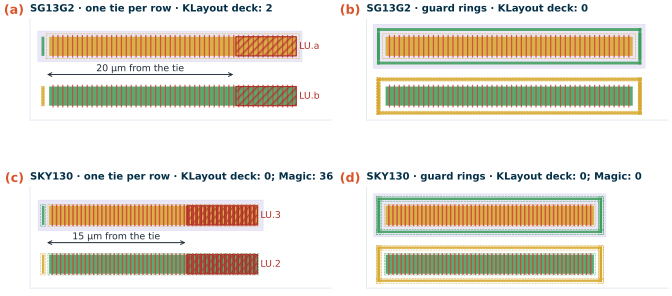
rel_layouts.py; contacts and first metal hidden. Hatched: the decks' latch-up markers. (a, c) One tie per row; (b, d) guard rings at 0.6 µm. Counts from IHP's KLayout deck (SG13G2), sky130A_mr.drc and Magic drc(full) (SKY130).Figure 24.6 shows the result. In SG13G2 the rows are 25.8 µm long, and both rules fire on the last 6.3 µm of each row, exactly the part more than 20 µm from the tie: one LU.b marker on the NMOS row and one LU.a marker on the PMOS row. In SKY130 the rows are 21.75 µm long and Magic marks everything beyond 14.4 µm, which is 15 µm from the centre of the tie’s contact, not from the edge of its active area. The SKY130 KLayout deck reports nothing, as in Chapter 23. With guard rings both layouts are clean in every deck, and every other rule of the decks passes too: the rings are drawn at the minimum widths, enclosures and implant overlaps of Table 23.4.
lu_ring, 30.1 × 11.1 µm: 0 violations in IHP's deck, including LU.a and LU.b.
lu_ring, 25.7 × 10.7 µm: 0 violations in Magic drc(full), including LU.2 and LU.3, and in sky130A_mr.drc.
What this means for your design
Put a guard ring around every group of devices, even where the rules would allow a single tie: it costs a strip of 0.30 µm (SG13G2) or 0.25 µm (SKY130) of active area and its spacing, it makes the latch-up rules pass by construction, and it buys a factor of thirty in trigger current. Place the n-well tie, or the n-well’s ring, on the side facing the NMOS devices, as in Figure 24.3. Near the pads, use double rings and keep the I/O devices well away from the core. The guard rings of the course OTA (Chapter 15) do exactly this, and they also keep substrate noise away from the matched devices of Chapter 27.
Try it · Find the longest row a single tie can protect
In
tools/layout/ch24/rel_layouts.py, setNF = 38and runpython3 tools/layout/ch24/rel_layouts.py. Before you look, compute the row length (Chapter 23’s gate pitch: 0.51 µm in SG13G2, 0.43 µm in SKY130, plus the two source/drain ends) and predict which PDK still fails. Then put the tie in the middle of the row instead of at its end, and find the largestNFthat passes in each PDK.
24.6 The antenna effect
The metal layers are patterned by plasma etching, and the plasma deposits charge on every conductor it touches (Chapter 17). A conductor connected to a diffusion drains the charge harmlessly through the junction. A conductor connected only to gates has no path except through the gate oxide: the charge collected by the conductor tunnels through the oxide of the gates it reaches, and if there is much charge and little gate, the current density can damage the oxide, shift the threshold voltage or create traps that later fail [61]. The damage is done during manufacture, long before the circuit is powered, and it is invisible to every simulation. The amount of charge grows with the area of the conductor exposed to the plasma (its top surface, or its etched sidewalls), and the damage per unit area of oxide falls with the gate area. Hence the antenna ratio
\[AR = \frac{A_{conductor}}{A_{gate}}, \tag{24.7}\]which the rules limit for each layer as it is etched. Once a higher layer connects the net to a diffusion, the hazard ends for every layer above.
The rules of both PDKs
Table 24.5. Antenna rules. SG13G2: layout rules sec. 7.1, cumulative areas [16]. SKY130: Magic sky130A.tech, extraction section ("model partial", each layer on its own) [20].
| Layer | SG13G2, max. ratio to gate area | SKY130, max. ratio to gate area |
|---|---|---|
| Poly over field | 200 (Ant.a), area | 50, sidewall area |
| Contacts | 20 (Ant.c), area | 3, area |
| li1 | — | 75, sidewall; with a diode 450 × diode area (µm²) |
| Metals | 200 cumulative, Metal1 to TopMetal2 (Ant.b) | 400 per layer, sidewall area (perimeter × thickness), met1 to met5 |
| Metals with a protection diode | 20 000 cumulative (Ant.e) | 2200 + 400 × diode area |
| Vias | 20 cumulative (Ant.d); 500 with a diode (Ant.f) | 3 (via), 6 (via2–via4); 18 or 36 × diode area with a diode |
| Protection diode | at least 0.16 µm² (Ant.g) | any diffusion that is not a transistor (“tiedown”) |
| Checked by | run_drc.py --antenna (not by default) |
Magic extract + antennacheck (check_antenna.py) |
The two decks differ in two ways that change the answer. SG13G2 counts top areas and accumulates them: the ratio at Metal3 is the Metal1 ratio, plus the Metal2 area connected to the gate at the Metal2 step, plus the Metal3 area, as IHP’s deck computes it layer by layer with the connectivity at each step. SKY130 counts the sidewall area of each layer on its own, because it is the etched sidewall that collects charge in its process; a wider wire then costs nothing more, only a longer one does. Both decks treat any diffusion on the gate’s net as protection. IHP’s deck looks for it on the finished net and then applies Ant.e instead of Ant.b; Magic treats a net that reaches any diffusion other than a transistor as tied down.
Worked example 24.3 · How long may a wire to a gate be?
A minimum NMOS (\(W\) = 1 µm, \(L\) = 0.13 µm in SG13G2, 0.15 µm in SKY130; Chapter 23’s hand-drawn transistor) has its gate wired through a Via1 to a long Metal2 / met2 wire, 0.3 µm wide, that leaves the block at an input pin. Nothing else is on the net inside the block.
SG13G2. \(A_{gate}\) = 0.13 µm². Ant.b allows a cumulative metal area of 200 × 0.13 = 26 µm². The Metal1 stub from the gate contact to the via is about 1 µm², so the Metal2 wire may have 25 µm², 83 µm of 0.3 µm wide wire (125 µm at the minimum width of 0.20 µm).
SKY130. \(A_{gate}\) = 0.15 µm². The met2 rule allows a sidewall area of 400 × 0.15 = 60 µm²; a wire of length \(\ell\) has \(2\ell\) of perimeter times 0.36 µm of thickness, so \(\ell\) ≤ 60 / 0.72 = 83 µm, whatever its width.
The generated wire (
ant_wireinrel_layouts.py) is a meander of eight 40 µm legs, 327 µm in total. By hand: SG13G2, the Metal2 area is 98.4 µm² (computed from the drawn rectangles), a ratio of 757, almost four times the limit; SKY130, the perimeter is about 656 µm, a sidewall area of 236 µm² and a ratio of 1574, four times the limit. The decks agree: IHP’s deck reports Ant.b at Metal2 and, because the ratio is cumulative, again at every layer above it up to TopMetal2 (six markers on the gate); Magic’s antenna check reports “Effective antenna ratio 1574.79 > limit 400” at plane metal2.
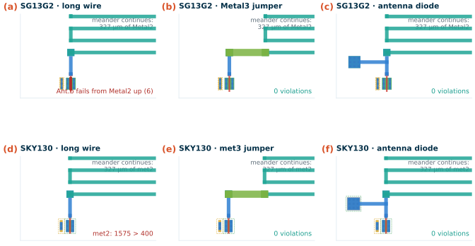
rel_layouts.py (the 327 µm Metal2/met2 meander continues to the right): (a, d) wire connected on Metal2; (b, e) a 3 µm Metal3/met3 jumper next to the gate; (c, f) an n+ diode of 1 µm² on the gate net. Results of IHP's deck with --antenna and of Magic's antennacheck; all three cells also pass the full DRC of both PDKs.Two fixes
A jumper. Break the long wire next to the gate and bridge the break on the next metal up (Figure 24.7b, e). While Metal2 is etched, the long wire is not yet connected to the gate; when Metal3 is etched, the long Metal2 is already buried under oxide and only the short bridge is exposed. Both decks agree: zero violations. The jumper costs two vias and a few micrometres of the next metal, and it works whatever is at the other end of the wire. Two details make it work: the bridge must be close to the gate (the piece of wire still attached to the gate is what counts), and it must go up: a jumper down to a lower metal exposes nothing less. A violation on the top metal cannot be jumpered at all.
A diode. Connect a small reverse-biased diode to the gate net on the lowest metal (Figure 24.7c, f). The diode is off in operation but conducts the plasma current during manufacture, by leakage or by breaking down, and keeps the gate voltage low. In SG13G2 the ratio limit rises to 20 000 (Ant.e), so the 757 of the example passes easily; in SKY130 Magic treats the diffusion as a tie-down and stops counting. Use the PDK’s antenna diode cell (dantenna and dpantenna in SG13G2, sky130_fd_pr__diode_pw2nd_05v5 in SKY130) in a real design, so that LVS recognizes it. The diode costs a junction capacitance and a leakage current on the gate net, which matter on a high-impedance analog node (a sample-and-hold capacitor, a floating-gate structure, an integrator input); there, prefer the jumper. The SG13G2 layout rules recommend a diode on every gate of circuits that are especially sensitive to threshold shifts and mismatch, such as sense amplifiers and some analog circuits [16].
Common pitfall · A clean block, a failing chip
Inside the block of Example 24.3 the input wire ends at a pin, and the block-level check sees a gate with a long wire and nothing else. At chip level the same wire may be connected to a driver’s drain and pass, or it may grow longer on its way to a pad and fail by a larger margin. The antenna check is a chip-level check in both PDKs (Chapter 17): run it on every block anyway, treat every input pin as unprotected, and fix the violations inside the block, where a jumper costs nothing, rather than at tape-out, where it may not fit.
Try it · Shorten the antenna
In
rel_layouts.py, setMEANDER = dict(legs=2, leg=40.0, pitch=1.0, w=0.3): 81 µm of wire. Predict the ratios with Example 24.3 before you run the script. Which deck passes, and by how much? Then make the wire wider (w=0.6) and explain why one deck changes its answer and the other does not.
24.7 Oxide stress and hot carriers
Two slow mechanisms wear out transistors that are used within their voltage limits, and both are why those limits come with a temperature and a lifetime.
Time-dependent dielectric breakdown (TDDB). A gate oxide under a field slowly accumulates traps. When enough of them line up, a conductive path forms and the oxide breaks down, after a time that falls exponentially with the field and with temperature [61]. That is why the core-device limit is a voltage at a temperature (SG13G2: 1.65 V at 125 °C, a field of 6.2 MV/cm across 2.65 nm), and why a small overvoltage held for a long time is dangerous even where a short one is harmless. A large MOS capacitor is the most exposed device: its whole area is under the full field all the time, and TDDB failures scale with area.
Hot-carrier injection (HCI). In a saturated transistor the carriers gain energy in the high field near the drain. A few gain enough to create interface traps or to be injected into the oxide, and the threshold voltage and transconductance drift over time. The damage is worst for NMOS devices at large \(V_{DS}\), short channel length, and a gate voltage of roughly half the drain voltage, where substrate current peaks [125]. Bias-temperature instability (NBTI) is its counterpart in PMOS devices: a negative gate bias at high temperature shifts the threshold even without drain current.
For the circuits of this course, three consequences follow.
- Analog bias points are mild. The OTA’s devices sit at \(V_{DS}\) of a few hundred millivolts and gate lengths of 0.5 to 5 µm, far from the worst case. Long channels also make the threshold shift matter less, because the lateral field is lower.
- Watch the devices that see the full supply with current. An output stage during slewing, a comparator’s latch, the switches of the switched-capacitor circuits and the charge pump of the PLL (Chapters 18–22) all pass through high \(V_{DS}\) with current flowing. Keep them at or above minimum length plus a margin, and use cascodes to share large voltages.
- Thick oxide where the voltage is high. Anything connected to a 3.3 V net (I/O, a higher analog supply, ESD clamps) belongs to the thick-oxide devices of Table 24.1, with their longer minimum length; a core device used there violates both TDDB and HCI limits at once.
- The gate oxide, not the junction, sets the hard voltage limit: SG13G2 core devices are qualified to 1.65 V at 125 °C (6.2 MV/cm across 2.65 nm), SKY130 core models to 1.95 V; junctions break down near 12 V in both PDKs.
- Electromigration follows Black’s equation, \(\mathrm{MTTF} \propto j^{-n} e^{E_a/kT}\): the allowed current halves for about every 20 K. SG13G2 publishes its limits (Metal1 1 mA/µm, Metal2–5 2 mA/µm, TopMetal1/2 15/16 mA/µm, Via1 0.4 mA, at 105 °C for 11 years); SKY130 publishes none, and our estimate scales SG13G2’s by cross-section.
- Analog bias currents fit in minimum-width wires (the OTA’s 60 µA output stage has a margin of 3 in SG13G2 at 125 °C); milliampere currents need micrometres of metal and tens of vias. No deck checks current density: you do.
- Heating limits the RMS current of the thick top metals (11 K for a 10 µm TopMetal2 at its DC limit) but not of the thin ones; device self-heating is negligible for the OTA (0.01 K) and not for a small HBT (11 kK/W).
- A CMOS inverter is a thyristor. With ties at the rule limits (20 µm, 15 µm) 0.17 mA of injected current latches it and it holds below 1 V; guard rings raise the trigger and holding currents about thirty-fold and pass LU.a/b and LU.2/3 in every deck.
- The antenna ratio of a gate on a long wire is easy to compute by hand (757 in SG13G2, 1574 in SKY130 for 327 µm of Metal2 on a minimum gate); the decks agree, and a jumper to the next metal or a diode fixes it. Run the antenna check: it is off by default in SG13G2.
Further reading
- R. A. Hastings, The Art of Analog Layout [61], the chapter on failure mechanisms: electrical overstress, electromigration, dielectric breakdown, the antenna effect, hot carriers and minority-carrier injection, with layout countermeasures for each.
- J. Lienig and M. Thiele, Fundamentals of Electromigration-Aware Integrated Circuit Design [68]: the physics behind current-density rules, Blech length, AC and pulsed currents, and how a design flow checks them.
- J. R. Black [123] and I. A. Blech [124]: the two classic papers on electromigration lifetime and the short-line effect.
- C. Hu et al. [125]: the hot-carrier degradation model that most reliability rules for MOSFETs still rest on.
- IHP, SG13G2 Process Specification [15] (sections 2.1–2.6 and 2.15) and Layout Rules [16] (section 7): the voltage, current-density, antenna and latch-up rules quoted here.