Chapter 25
Resistors
Integrated resistors are rectangles of resistive film, and almost every way they deviate from their nominal value can be traced to their layout: contacts, width, bends, temperature, voltage and the substrate beneath. This chapter takes the resistors of SG13G2 and SKY130 apart, one effect at a time, with the PDKs' own generators and models.
- Calculate a resistor from sheet resistance, square count, width bias and head resistance, including bends and serpentines.
- Read the layout of a resistor head and body in both PDKs, and say which edge defines the resistor’s length.
- Quantify width bias, temperature and voltage coefficients from the PDK models, and explain how the layout changes them.
- Estimate the capacitance and the distributed-RC bandwidth of a long resistor, and know when the PDK model is not enough.
- Choose between the resistors of SG13G2 and SKY130 for a given job, and design a trim network that absorbs their process spread.
Contents
- 25.1 Sheet resistance and the square count
- 25.2 Resistor layout: bodies, heads and contacts
- 25.3 Variability: width bias, temperature and voltage coefficients
- 25.4 Parasitics: capacitance to substrate and distributed RC
- 25.5 The resistors of SG13G2 and SKY130 compared
- 25.6 Trimming and adjustable resistors
- Further reading
Chapter 3 listed the resistors of both PDKs and extracted their sheet resistance, width bias and end resistance from the models (Eq. 3.2 and Worked example 3.1); Chapter 15 placed one as the nulling resistor of the course OTA; Chapter 13 gave its thermal noise. This chapter goes underneath those numbers. It asks where each term of the resistance comes from in the layout, how a bend or a head changes it, how temperature, voltage and the substrate move it, and what to do when the process spread is larger than the circuit tolerates. Matching of resistor pairs, with common-centroid arrays and dummies, is the subject of Chapter 27. The layouts come from the PDKs’ own generators (IHP’s KLayout PyCells and Magic’s SKY130 device generators), the numbers from the PDK documents and from ngspice runs of the PDK models in IIC-OSIC-TOOLS [35]:
python3 tools/layout/ch25/res_layouts.py     # PyCells and Magic draw the resistors; GDS, extraction, 3D model
python3 tools/figs/_ch25_sim.py              # resistor simulations in both PDKs (a few minutes)
python3 tools/figs/ch25_resistors.py         # the figures and tools/figs/ch25_numbers.json
25.1 Sheet resistance and the square count
A uniform film of resistivity \(\rho\) and thickness \(t\), cut into a rectangle of length \(L\) (along the current) and width \(W\), has the resistance \(R = \rho L/(tW)\). The process fixes \(\rho\) and \(t\); the layout fixes only \(L\) and \(W\). So the two are separated into the sheet resistance
\[R_\square = \frac{\rho}{t}, \qquad R = R_\square\,\frac{L}{W} = R_\square\,N, \tag{25.1}\]where \(N = L/W\) is the number of squares. Any square of the film, whatever its size, has the same resistance \(R_\square\) between two opposite edges: doubling the side doubles the length and the cross-section together. That is why sheet resistance is quoted in ohms per square (Ω/□), and why a resistor’s value is a count of squares, not of micrometres.
The materials differ by almost three orders of magnitude in sheet resistance, for physical reasons that also set their temperature behaviour (Section 25.3):
- Salicided poly (SG13G2
rsil, 7 Ω/□) is gate polysilicon with a metal silicide formed on top. The silicide carries almost all the current, so the film behaves like a metal. - Doped, unsalicided poly (SG13G2
rppd, 260 Ω/□; SKY130res_high_po, about 320 Ω/□) keeps the silicide off with a block layer and conducts through the heavily doped polysilicon itself. SKY130’sres_generic_po(48 Ω/□) is ordinary gate polysilicon, drawn as a resistor. - Lightly doped poly (SG13G2
rhigh, 1360 Ω/□; SKY130res_xhigh_po, 2000 Ω/□) has so few free carriers that the energy barriers at its grain boundaries, not the grains themselves, set the resistance. - Diffusions and wells (SKY130
res_generic_nd120 Ω/□,res_generic_pd197 Ω/□, the n-well 1.7 kΩ/□ and the isolated p-wellres_iso_pw3.8 kΩ/□) are doped regions of the silicon, isolated from their surroundings by a reverse-biased junction. SG13G2 offers no characterized diffusion or well resistor; its three poly resistors span the whole range [15, 19].
Figure 25.1 shows all of them as the generators draw them, at one scale.
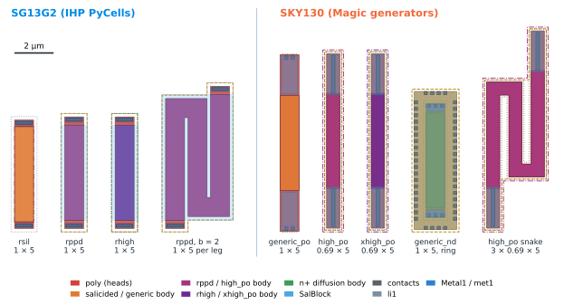
b = 2 option and Magic's nx = 3, snake = 1. Generated by tools/layout/ch25/res_layouts.py; colours as in the 3D gallery.Counting squares around corners
Equation (25.1) assumes the current flows straight and uniformly. In a bend it does not: it crowds towards the inner corner, where the path is shortest, and hardly uses the outer corner at all. The resistance of a bent strip therefore cannot be found by counting the squares along its centreline. It has to be found from the potential in the film, which obeys Laplace’s equation \(\nabla^2 V = 0\) inside the shape, with no current crossing its edges and the two terminals held at fixed potentials. The number of squares is then \(N = 1/I\) for a film of unit sheet conductance at 1 V.
tools/figs/_ch25_squares.py solves this on a fine grid for any polygon (a 40-line finite-volume solver with conjugate gradients, checked on a straight strip, which it reproduces to four digits). Figure 25.2 shows the result for the two shapes every serpentine is made of:
- A right-angle corner of equal widths counts 0.558 squares, not one and not a half. This matches the classic thin-film result that Hastings quotes, 0.5587 [61]; the rule of thumb “a corner counts half a square” is 10 % low, and counting the corner as a full square is 79 % high.
- A U-turn (two corners joined by a short straight piece) counts slightly less than two corners plus the gap: 2.11 squares for a gap equal to the width, against 2 × 0.558 + 1 = 2.12; for the tight gap of an SG13G2 PyCell serpentine (s/W = 0.18) the turn counts 1.22 squares, 0.08 less than the sum of its parts, because the two inner corners share their crowded region.
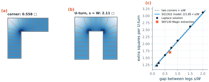
Both PDKs build this knowledge into their tools. The SG13G2 rppd and rhigh models take the number of bends b as an instance parameter and lengthen the resistor by \(2W/1.85 + s\) per bend (that is, 1.08 squares plus the gap; Figure 25.2c, blue line), within 4 % of the Laplace solution over the whole range [14]. Magic computes the length of a snake when it extracts it; Worked example 25.1 checks both against the layouts of Figure 25.1.
The complete layout equation
Combining the square count with the two corrections of Chapter 3 (the width bias \(\Delta W\) and the head resistance) gives the equation used for the rest of this chapter:
\[R = R_\square\left(\frac{L}{W+\Delta W} + n_U N_U\right) + 2R_h, \tag{25.2}\]where \(L\) is the total length of the straight legs, \(n_U\) the number of U-turns, \(N_U\) the squares of each turn from Figure 25.2c, and \(R_h\) the resistance of one head (contact, silicide-to-poly interface and the head’s own film). Each term belongs to a different part of the layout, and each varies in its own way: \(R_\square\) with the film’s doping and thickness, \(\Delta W\) with lithography and etch, \(R_h\) with the contact process. Section 25.3 follows them one by one.
25.2 Resistor layout: bodies, heads and contacts
Which edge defines L
The drawn length of a resistor is not the length of its poly. It is the length of the region with the body’s sheet resistance, and that region is defined by a marker layer, not by the contacts:
- SG13G2
rppdandrhigh: L is the length of the salicide block (SalBlock) over the poly. Outside it the poly is silicided and nearly a short circuit (7 Ω/□). The rules fix the SalBlock edge to the contact at exactly 0.20 µm (Rppd.c and Rhi.d are “min. and max.”), so the silicided gap between contact and body has the same length in every resistor and its resistance becomes part of the calibrated head [16]. Forrsilthe resistor marker RES defines L, at least 0.12 µm from the contacts (Rsil.b). - SKY130 precision resistors: L is the length of the poly under the resistor marker
poly.res(66/13) between the two heads. Each head is 2.08 µm long and carries a single slot contact of 0.19 × 2.00 µm; the whole device sits under therpm(orurpm) implant layer [20, 18].
Figure 25.3 zooms into one head of each.
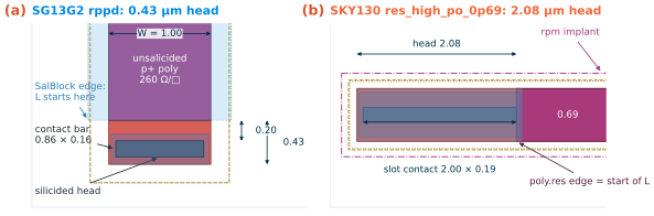
rppd, W = 1 µm: the contact bar sits exactly 0.20 µm from the SalBlock edge (Rppd.c). (b) SKY130 res_high_po_0p69: a 2.08 µm head with a 2 µm slot contact before the poly.res marker begins. Same scale in both panels; dimensions in µm, read from the generated GDS.The two heads cost very different amounts of resistance. In SG13G2 the specification gives the “metal-to-body resistance” per micrometre of width: 4.5 Ω·µm for rsil, 35 Ω·µm for rppd and 80 Ω·µm for rhigh, and the models reproduce them exactly (fits of 4.5, 35.2 and 78 Ω·µm) [15]. For a 1 µm wide rppd the head is worth 35 Ω, the resistance of only 0.13 µm of body. SKY130’s precision heads are far larger: about 195 Ω per head for the 0.69 µm width (the model’s rcon of 390 Ω covers both), 304 Ω at 0.35 µm and 34 Ω at 5.73 µm, which is 106 to 195 Ω·µm, or the resistance of 0.4 µm of body at the 0.69 µm width (Figure 25.4b) [19]. The generic SKY130 resistors (res_generic_po, res_generic_nd) are modelled with no head resistance at all.
Table 25.1. The layout of the resistor devices, from the generated cells and the rule documents [16, 20, 19].
| Device | L defined by | Head | Minimum W / L (µm) | Width |
|---|---|---|---|---|
SG13G2 rsil |
RES marker on GatPoly | contact bar, ≥ 0.12 from RES | 0.5 / 0.5 (Rsil.a, f) | any |
SG13G2 rppd |
SalBlock over p+ poly | 0.43 µm, bar exactly 0.20 from SalBlock | 0.5 / 0.5 (Rppd.a, e) | any; ≥ 2 recommended for precision |
SG13G2 rhigh |
SalBlock over p+ and n+ implanted poly | as rppd |
0.5 / 0.5 (Rhi.a, f) | any |
SKY130 res_generic_po |
poly.res marker |
contacts on the poly end | 0.33 / 1.65 | any |
SKY130 res_high_po_* |
poly.res under rpm |
2.08 µm, one 0.19 × 2.00 slot | fixed / 0.5 | 0.35, 0.69, 1.41, 2.85, 5.73 |
SKY130 res_xhigh_po_* |
poly.res under urpm |
as res_high_po |
fixed / 0.5 | 0.35, 0.69, 1.41, 2.85, 5.73 |
SKY130 res_generic_nd |
resistor marker on n+ diff (65/13) | diffusion contacts | 0.42 / 2.1 | any; tap ring around |
SKY130 res_iso_pw |
p-well resistor marker (64/13) in a deep n-well | well contacts | 2.65 / 26.5 | fixed 2.65 |
Strip, dogbone and the current in the head
A head can be as wide as the body (a strip resistor) or wider (a dogbone). Where the contact is narrower than the strip, the current must squeeze into it and the resistor reads slightly high; where the head is wider than the body, the current spreads out and it reads slightly low [61]. Both PDKs avoid the question by making every head the width of its body: SG13G2 puts a contact bar across the full width (0.86 µm in a 1 µm resistor, 0.07 µm in from each side), and SKY130 a slot along the head. Whatever residual effect remains is the same in every resistor of a given width and is already inside the calibrated head resistance. The rule for a layout is therefore simple: draw resistors with the generator, and do not edit the heads. A contact moved, added or removed changes \(R_h\), which the model no longer knows.
Serpentines and turns
A long resistor is folded into legs to keep its outline compact. Three layout rules follow from Section 25.1:
- Count every turn. Each U-turn adds \(N_U\) squares (Figure 25.2c). Use the generator’s bend parameter (
bin SG13G2) or let the extraction count them (Magic in SKY130); never feed the straight length alone into the model. - For matching, prefer straight segments joined in metal. Turns crowd the current into the inner corners, where the edge variation of the film matters most. A resistor made of identical straight segments connected by metal has no turns, and every segment has the same orientation and the same heads (Chapter 27). The cost is two heads per segment, which in SKY130 is not small.
- Mind the voltage between adjacent legs. Legs of a serpentine run side by side at the poly spacing (0.18 µm in the SG13G2 PyCell). The voltage between adjacent legs is a fraction of the total, at most \(2V/N\) for N equal segments; it is small for a resistor at the 1.2 V or 1.8 V core supply, but a high-voltage divider needs spacings that grow with that voltage [61].
The SG13G2 serpentine of Figure 25.1 as a 3D model, built from the PyCell’s GDS with tools/3d/gds2glb.py. Hide the SalBlock to see that the whole serpentine, turns included, is one unsalicided body, and that only the short heads at the two ends are silicided.
IHP PyCell rppd, w = 1 µm, l = 5 µm, b = 2: 17.45 squares by the Laplace solution, 17.52 by the model's bend formula.
Worked example 25.1 · The squares of a serpentine, by hand, against the generators
SG13G2, PyCell
rppdwith w = 1 µm, l = 5 µm, b = 2 (Figure 25.1). Reading the GDS, the three legs between the inner edges of the turns are 5.395, 4.195 and 5.410 µm long: the PyCell distributes \((b+1)\,l\) = 15.00 µm of straight body over the legs. The gap between legs is the poly spacing, s = 0.18 µm, so s/W = 0.18. With Eq. (25.2) and the corner rule:
- “half a square per corner”: N = 15.00 + 2 × (2 × 0.5 + 0.18) = 17.36
- “0.558 per corner” (two corners plus the gap): N = 15.00 + 2 × (1.116 + 0.18) = 17.59
- Laplace value of a U-turn at s/W = 0.18, 1.219: N = 15.00 + 2 × 1.219 = 17.44
The Laplace solution of the whole serpentine polygon gives 17.45 squares and the SG13G2 model, from its bend formula, 15 + 2 × (1.081 + 0.18) = 17.52 at the drawn width. The model is 0.4 % high; the simple rules bracket the answer within ±0.8 %.
SKY130, Magic
res_high_po_0p69with l = 5, nx = 3, snake = 1. The legs between the inner edges of the turns are 4.91, 3.62 and 4.91 µm (13.44 µm, 19.48 squares), the gap 0.48 µm (s/W = 0.70), and each turn counts 1.81 squares in the Laplace solution. By hand, N = 19.48 + 2 × 1.81 = 23.10 squares; the Laplace solution of the full polygon gives 23.08. Magic’s extraction reportsl=15.78, that is 15.78/0.69 = 22.87 squares: Magic credits each turn with 1.70 squares instead of 1.81, and its value is 0.9 % low. At about 340 Ω per drawn square of this width, that is 70 Ω out of 8.2 kΩ: irrelevant for a ratio of two identical snakes, but an error of the absolute value that no corner of the model covers.
25.3 Variability: width bias, temperature and voltage coefficients
A resistor’s value moves with the process (from wafer to wafer), with temperature (during operation) and with the voltages on and around it. Each term of Eq. (25.2) responds differently, which is why the layout decides how much of each effect a resistor sees.
Process spread
The sheet resistance is the least controlled term. The SG13G2 specification accepts rsil between 6.2 and 7.8 Ω/□, rppd between 235 and 285 Ω/□ (±9.6 %) and rhigh between 1160 and 1560 Ω/□ (±15 %); the resistor corners res_bcs and res_wcs combine these limits with a width bias shifted by ±30 nm (rppd) or ±40 nm (rhigh) [15, 14]. SKY130’s resistor corners (ll, hh in the model library) move a 10 kΩ res_high_po network by ±14.5 % (Worked example 25.3) [19]. These are absolute tolerances. Two identical resistors side by side track each other to a fraction of a per cent (Chapter 27), which is why analog circuits are designed to depend on resistor ratios, and why an absolute value has to be trimmed (Section 25.6).
Lightly doped poly is the most variable film, because its resistance depends on the grain structure as much as on the doping. Boron-doped poly can also drift over the years at high temperature, as hydrogen that passivated its grain boundaries is lost [61]. Neither effect is in the models; both argue for the medium-sheet films (rppd, res_high_po) where precision matters.
Width bias
The film’s real width differs from the drawn width by the width bias \(\Delta W\): lithography and etch move both edges of the strip, and the implants of a doped film spread sideways. Because \(\Delta W\) is a fixed number of nanometres, its relative effect grows as the resistor gets narrower. Figure 25.4a extracts it from the models at two lengths and eight widths, removing the heads by taking the difference between the two lengths.
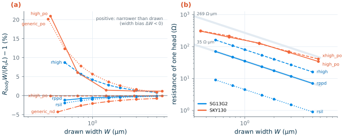
- SG13G2 follows Eq. (25.2) exactly, with the specification’s values: \(\Delta W\) = +10 nm (
rsil), +6 nm (rppd) and −40 nm (rhigh) [15]. A minimum-widthrhigh(0.5 µm) is 8.7 % above \(R_\square L/W\); at 2 µm the error is 2 %. - SKY130’s
res_high_pocomes as five separately characterized widths, and a single width bias describes them only roughly (−37 nm over all five). The 0.35 µm version is 21 % above the nominal 320 Ω/□, the 0.69 µm version 6 %, the wider ones about 1 %.res_generic_pohas \(\Delta W\) = −56 nm, so its 0.33 µm minimum is 20 % high.res_xhigh_pois modelled with no width bias at all, and the n+ diffusion with +17 nm (the diffusion spreads sideways) [19].
Width bias is a systematic error, which a hand calculation with \(\Delta W\) removes. Its variation is not: the edges of a narrow film wander by a few nanometres from one resistor to the next, and that random part sets matching (Chapter 27). Both reasons point the same way. IHP recommends at least 2 µm for precision rppd resistors [15]; a reasonable default in either PDK is a width two to four times the minimum, unless the resistor must be very large.
Temperature
The resistance of most films rises with temperature, because carriers scatter more often on a vibrating lattice and their mobility falls. Lightly doped poly is the exception: its current must cross the potential barriers at the grain boundaries, and more carriers do so when they are hot, so its resistance falls with temperature [61]. A quadratic fit around \(T_0\) is the PDKs’ description:
\[R(T) = R(T_0)\left[1 + TC_1\,(T-T_0) + TC_2\,(T-T_0)^2\right]. \tag{25.3}\]Figure 25.5a shows every resistor of both PDKs from −40 to 125 °C, and Table 25.2 the coefficients fitted to the simulations.
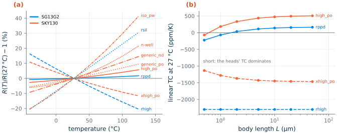
Table 25.2. Variability of the resistors: specification or model values, and coefficients fitted to the simulations of Figures 25.4 to 25.6 (L = 10 µm unless noted) [15, 19].
| Device | \(R_\square\) (Ω/□) | Spread | \(\Delta W\) (nm) | \(TC_1\) (ppm/K) | \(TC_2\) (ppm/K²) | Voltage dependence |
|---|---|---|---|---|---|---|
SG13G2 rsil |
7.0 | 6.2–7.8 | +10 | +3100 | 0.3 | none modelled |
SG13G2 rppd |
260 | 235–285 | +6 | +170 body, −950 head; +140 at L = 10 | 0.4 | self-heating only |
SG13G2 rhigh |
1360 | 1160–1560 | −40 | −2300 | 2.1 | self-heating only |
SKY130 res_generic_po |
48.2 | corners | −56 | +889 | 0.85 | none modelled |
SKY130 res_high_po_0p69 |
≈ 320 | ±14.5 % | ≈ −37 | +514 body; +474 at L = 10 | 1.1 | +0.26 % at 3 V |
SKY130 res_xhigh_po_0p69 |
2000 | corners | 0 | −1470 body; −1449 at L = 10 | 2.7 | −0.07 % at 3 V |
SKY130 res_generic_nd |
120 | corners | +17 | +1424 | 0.66 | none modelled |
| SKY130 n-well | 1700 | corners | — | +1442 | 7.9 | none modelled |
SKY130 res_iso_pw |
3816 | corners | — | +3525 | 7.3 | −1.3 %/V across, +3.0 %/V body |
The heads have their own temperature coefficient, and in a short resistor they matter. In SG13G2 the rppd body has +170 ppm/K but its heads −950 ppm/K (the specification’s TC3, the temperature coefficient of the metal-to-body resistance) [15]. The resistor’s coefficient is the resistance-weighted mean of the two,
so it falls from +164 ppm/K for a 50 µm rppd to −223 ppm/K for a 0.5 µm one (Figure 25.5b). In SKY130 the head resistance has no temperature coefficient in the model, which pulls res_high_po from +506 ppm/K (long) to −69 ppm/K (0.5 µm), and res_xhigh_po from −1466 to −1135 ppm/K. SG13G2’s rhigh has the same coefficient in body and head and stays at −2300 ppm/K at every length.
What this means for your design
The temperature coefficient is partly a layout parameter. Two consequences are worth using. First, resistors that must track over temperature must have the same length, not just the same material: a 2 kΩ
rppdmade of two short segments and a 20 kΩ one made of one long strip differ by 100 ppm/K or more, a 1.6 % ratio error over −40 to 125 °C. Build both from identical unit segments. Second, opposite coefficients can be combined: in SKY130,res_high_po(+474 ppm/K) in series withres_xhigh_po(−1449 ppm/K) in a resistance ratio of about 3 : 1 gives a composite with nearly zero first-order coefficient; in SG13G2,rppdalone is already within ±200 ppm/K, and long segments keep it there.
Voltage
An ideal resistor is linear: its value does not depend on the voltage across it. Real films deviate for three reasons [61]:
- Self-heating. The power \(V^2/R\) warms the film, and the temperature coefficient turns the temperature rise into a resistance change. Poly sits on oxide, a poor heat conductor, so it heats more than a diffusion of the same size. The SG13G2 models include a thermal network that is switched on with the instance parameter
sw_et=1. - Field effects in the film. At high fields, carriers in a short resistor approach velocity saturation, and in poly the voltage drop across each grain boundary changes its barrier. Both make long resistors more linear than short ones.
- Depletion from the body. A diffused or well resistor is separated from its surroundings by a reverse-biased junction. The depletion region of that junction eats into the conducting layer, more where the reverse bias is larger, so the resistance depends on the voltage between the resistor and its body. This body (or conductivity) modulation is the diffused resistor’s equivalent of the MOSFET’s body effect. Poly resistors are isolated by oxide and do not have it.
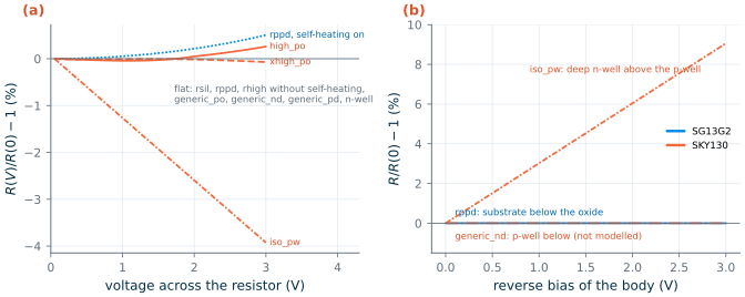
rppd, W = 1 µm, with the model's self-heating switched on. (b) Against the reverse bias between resistor and body, 0.1 V across the resistor.Figure 25.6 shows how the models treat each mechanism. The SG13G2 poly resistors are linear to 0.01 % at 3 V. With self-heating switched on, a 1 × 10 µm rppd at 3 V carries 1.13 mA, close to the specification’s 1.2 mA/µm limit, dissipates 3.4 mW and rises by +0.51 %: with its coefficient of +140 ppm/K, a temperature rise of about 35 K. An rhigh heated by the same 35 K would fall by 8 %, so self-heating is a real nonlinearity for high-value resistors carrying signal current; Chapter 24 treats the heating itself. SKY130’s precision poly models carry explicit voltage terms, +0.26 % at 3 V for res_high_po and −0.07 % for res_xhigh_po. The isolated p-well resistor res_iso_pw shows body modulation in full: −1.3 % per volt across it and +3.0 % per volt of reverse bias from its deep n-well, as its model’s coefficients say [19].
Common pitfall · Trusting a linear model of a diffused resistor
SKY130’s
res_generic_nd,res_generic_pdand n-well resistor are modelled as plain resistors with junction diodes to their body. They show no dependence on the voltage across them or on the body bias (Figure 25.6b), but the physical devices have the same depletion mechanism asres_iso_pw, whose model shows 3 %/V. A divider or a gain-setting resistor made from them will be nonlinear on silicon while the simulation stays perfect. Use poly for anything that must be linear; if you must use a diffusion or a well, keep the voltage across each segment small, give every segment its own body tied to its own upper end so that all segments see the same reverse bias [61], and ask whether the model contains the effect before you trust its answer.
25.4 Parasitics: capacitance to substrate and distributed RC
The capacitance of a resistor
A poly resistor is a plate above the substrate, separated from it by the trench oxide. Its capacitance has an area term and a fringe term along both long edges, and the models give both:
- SG13G2: 0.09 fF/µm² and 0.025 fF/µm per edge, applied over the body plus 0.86 µm of head (
ca,cp,lheadin the r3_cmc models) [14]. A 0.5 µm widerhighhas 95 aF per micrometre of length. - SKY130: 0.106 fF/µm² and 0.054 fF/µm per edge (0.050 for
res_xhigh_po), over the body plus both 2.08 µm heads [19]. A 0.69 µmres_xhigh_pohas 174 aF/µm: the fringe term is twice SG13G2’s, and at this width it dominates.
A diffused resistor adds a junction to its body instead: SKY130’s res_generic_nd model puts a diode of half the body area at each terminal, whose capacitance falls with reverse bias and whose leakage rises with temperature.
The distributed RC line
The capacitance is not at the ends of the resistor; it is spread uniformly along it. A long resistor is a distributed RC line, and its response is not that of a single pole. Both PDK models, however, lump the capacitance into a π: half of it at each terminal. The difference matters exactly when the resistor is long and the frequency high.
Derivation · The bandwidth of an open-ended RC line
Let the line have total resistance \(R\) and total capacitance \(C\), spread over its length, with \(x\) running from the driven end (0) to the open end (1). The current \(i(x)\) and voltage \(v(x)\) obey, in the Laplace domain,
\[\frac{dv}{dx} = -R\,i, \qquad \frac{di}{dx} = -sC\,v,\]so \(d^2v/dx^2 = sRC\,v\). With \(\gamma = \sqrt{sRC}\), the solution that satisfies \(v(0) = V_{in}\) and no current at the open end, \(dv/dx\,(1) = 0\), is \(v(x) = V_{in}\cosh(\gamma(1-x))/\cosh\gamma\). At the open end,
\[H(s) = \frac{V_{out}}{V_{in}} = \frac{1}{\cosh\sqrt{sRC}}. \tag{25.5}\]Setting \(\lvert H(j\omega)\rvert = 1/\sqrt{2}\) and solving numerically gives \(\omega RC = 2.43\). The π model has only its far-end capacitor \(C/2\) in the signal path, \(H = 1/(1 + sRC/2)\), with \(\omega RC = 2\) at −3 dB. Beyond the corner the two separate quickly: the π model falls at 20 dB per decade, the real line much faster (and with far more phase shift), because every piece of the line is a further low-pass section.
The −3 dB bandwidth of a resistor driven at one end and open at the other is therefore
\[f_{3dB} = \frac{2.43}{2\pi RC} \quad\text{(distributed)}, \qquad f_{3dB,\pi} = \frac{2}{2\pi RC} \quad\text{(PDK model)}. \tag{25.6}\]For a resistor of given value, the layout sets \(C\). With \(L = R(W+\Delta W)/R_\square\) and a capacitance \(c'\) per unit length, \(RC = R^2 c'\,(W+\Delta W)/R_\square\): the time constant grows with the square of the resistance, and falls with higher sheet resistance and narrower width. That is the opposite of what matching wants, which is the trade-off of every high-value resistor.
Worked example 25.2 · How fast is 100 kΩ of high-sheet poly?
SG13G2,
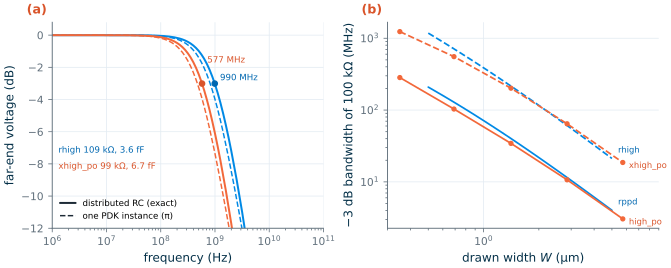
rhigh, W = 0.5 µm, L = 36.7 µm. With Eq. (25.2): \(R\) = 1360 × 36.7/(0.5 − 0.040) + 2 × 80/0.5 = 108.5 k + 0.3 k = 108.8 kΩ (the width bias alone adds 8.7 %). The capacitance per micrometre is 0.09 × 0.5 + 2 × 0.025 = 0.095 fF/µm, over 36.7 + 0.86 µm: \(C\) = 3.57 fF. Then \(f_{3dB}\) = 2.43/(2π × 108.8 kΩ × 3.57 fF) = 996 MHz.SKY130,
res_xhigh_po_0p69, L = 34.2 µm. \(R\) = 2000 × 34.2/0.69 + 2 × 202 = 99.5 kΩ. The capacitance covers the body and both heads, 34.2 + 4.16 = 38.36 µm: area 0.106 × 0.69 × 38.36 = 2.81 fF, fringe 0.050 × 2 × (38.36 + 0.69) = 3.90 fF, \(C\) = 6.71 fF. Then \(f_{3dB}\) = 2.43/(2π × 99.5 kΩ × 6.71 fF) = 579 MHz.Simulation. The models give 108.8 kΩ and 3.59 fF, and 99.5 kΩ and 6.74 fF, so the distributed bandwidths are 990 and 577 MHz (Figure 25.7a), within 1 % of the hand values. A single PDK instance puts the −3 dB point at 794 and 501 MHz instead, 20 % and 13 % low, and beyond it the phase is wrong by tens of degrees. For a feedback resistor or an RC filter near these frequencies, split the resistor into ten or more pieces in simulation (with ideal resistors and capacitors from the same R and C), or extract the layout with distributed parasitics (Chapter 16).
Same value, other material. In
rppd(W = 1 µm) the same 100 kΩ needs 387 µm of length and has a bandwidth of about 70 MHz; Figure 25.7b shows that every doubling of width costs another factor of about three.
Coupling through the substrate and from above
The same capacitance couples the resistor to whatever lies under it. Noise on the substrate (from digital circuits, switching regulators or the ground return of a power stage) reaches a high-impedance resistor node through it, and at 100 kΩ and a few femtofarads the corner of that coupling is a few hundred megahertz: well within the spectrum of digital edges. Three layout measures help [61]:
- Shield from below with an n-well under the resistor, tied to the quiet reference of the circuit the resistor belongs to, and surround it with a substrate tie ring connected to the same quiet ground (Chapter 24 for rings). The shield’s own capacitance to the substrate then carries the noise current instead of the resistor.
- Do not route signals over a resistor. A wire across it adds a coupling capacitance in series with the body; a digital line over a feedback resistor is the classic way to inject clock into an amplifier.
- Keep high-value resistors small and compact. Folding a long resistor into a square serpentine shortens nothing electrically, but it keeps the resistor away from distant aggressors and inside one guard ring.
25.5 The resistors of SG13G2 and SKY130 compared
Table 25.3 puts the numbers of this chapter side by side, with the job each resistor does best.
Table 25.3. Choosing a resistor: sheet resistance, head, capacitance and typical use (values from Sections 25.1–25.4) [15, 19].
| Job | SG13G2 | SKY130 |
|---|---|---|
| Very low values (< 100 Ω), gate and well straps | rsil, 7 Ω/□, +3100 ppm/K, head 4.5 Ω·µm; or metal |
res_generic_po, 48 Ω/□, +889 ppm/K; li1 at 12.8 Ω/□; or metal |
| Precision, ratios, feedback (0.5–50 kΩ) | rppd, 260 Ω/□, +170 ppm/K, head 35 Ω·µm, any width ≥ 0.5 µm |
res_high_po, ≈ 320 Ω/□, +514 ppm/K, heads 34–304 Ω, five widths |
| High values (50 kΩ–10 MΩ), bias networks | rhigh, 1360 Ω/□, −2300 ppm/K, ±15 % |
res_xhigh_po, 2000 Ω/□, −1470 ppm/K |
| Capacitance per µm at W = 1 µm | 0.14 fF/µm | 0.21 fF/µm (high_po heads add 2 × 2.08 µm) |
| Diffused or well resistors (ESD ballast, high power density) | none characterized | res_generic_nd/pd (120/197 Ω/□), n-well (1.7 kΩ/□), res_iso_pw (3.8 kΩ/□) |
| Maximum current density | rppd 1.2 mA/µm, rhigh 0.6 mA/µm (11 years, 105 °C) |
not given in the models |
SG13G2 vs SKY130 · The same 10 kΩ, two different resistors
For 10 kΩ of medium-sheet poly at 2 µm width, SG13G2’s
rppdneeds 77 µm and has two heads of 17.5 Ω each (0.35 % of the value). SKY130’sres_high_pocomes in 1.41 or 2.85 µm, not 2 µm; at 1.41 µm it needs 42 µm and its two heads are 256 Ω (2.6 %). The SKY130 head therefore dominates any short segment: the 175 Ω step of a trim network cannot be built fromres_high_po_0p69at all, whose two heads alone are 390 Ω (Worked example 25.3). SG13G2’s arbitrary widths and small heads make it the easier process for resistor networks; SKY130’s fixed widths are characterized individually, so a design that sticks to them gets accurate models, and its diffused and well resistors offer options SG13G2 does not have.
A few guidelines summarize the chapter so far:
- Use ratios, not absolute values. Make the circuit depend on the ratio of two resistors of the same material, width and segment length, and the process spread and most of the temperature coefficient cancel.
- Use the medium-sheet film for precision (
rppd,res_high_po): small width bias, small TC, low noise (Chapter 13). Use the high-sheet film only where area or capacitance forbids the medium one, and expect ±15 % and a large negative TC. - Width two to four times the minimum for anything that must be accurate; minimum width only for values that do not matter.
- Long segments, so that heads are a small part of the value and its temperature coefficient (Eq. 25.4).
- Poly for linearity; diffusions and wells only where their junction (ESD, power) is wanted.
25.6 Trimming and adjustable resistors
When a circuit needs an absolute value that the ±10 to ±15 % spread of Section 25.3 cannot deliver (a bandgap’s output, an on-chip termination, an RC time constant), the value must be adjusted after fabrication. There are two families of adjustment [61]:
- Tweaking changes the design for all future wafers: the first silicon is measured and one mask is changed. A resistor built from segments with spare ones in reserve, connected or bypassed in metal, can be tweaked by redrawing one metal layer; leaving those metal options in the layout from the start is cheap insurance for any value you are not sure of. (Sliding a contact along the body, the classic tweak for diffused resistors, does not work for salicide-blocked poly, whose length is fixed by the block layer.)
- Trimming adjusts each chip individually at test. Fuses, Zener zaps and laser trimming change the resistor permanently, but need process options and test equipment that a multi-project run rarely provides. Neither open PDK offers one: SG13G2 ships no fuse among its PyCells and libraries, and SKY130’s Magic technology file names a metal fuse device,
sky130_fd_pr__fuse_m4, but the open PDK provides no model, layout cell or programming conditions for it [14, 20]. The practical choice with open PDKs is a digital trim: segments of the resistor are shorted by MOS switches, whose gates are set by a register loaded at power-up or by a small one-time-programmable memory.
Designing a binary trim network
A trimmed resistor of target value \(R_t\) consists of a fixed part \(R_{fix}\) and \(n\) binary-weighted segments \(R_{LSB}, 2R_{LSB}, \ldots, 2^{n-1}R_{LSB}\), each shorted by a switch when its bit is 0. The process multiplies every value by a factor \(k\) between \(k_{min}\) and \(k_{max}\). Two conditions fix the design. At the highest-resistance corner with every segment shorted, the network must not exceed the target, and at the lowest-resistance corner with every segment in, it must reach it:
\[k_{max}\,(R_{fix} + R_{sw}) \le R_t \le k_{min}\left(R_{fix} + (2^n-1)\,R_{LSB}\right), \tag{25.7}\]where \(R_{sw}\) is what the closed switches leave in series. The step is \(k R_{LSB}\), so after trimming the error is at most half of it: \(\pm k_{max}R_{LSB}/(2R_t)\).
Worked example 25.3 · A 4-bit trim for 10 kΩ ± 1 % in both PDKs
SG13G2,
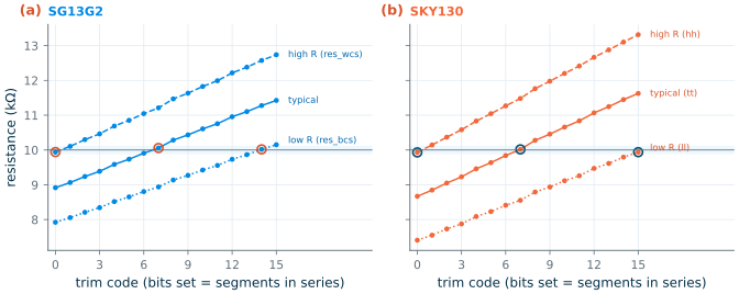
rppdW = 2 µm. The corners move \(R_\square\) by ±10 % and the width bias by ∓30 nm, so \(k_{max}\) = 1.10 × 2.006/1.976 = 1.117 and \(k_{min}\) = 0.90 × 2.006/2.036 = 0.887. Allowing about 100 Ω for four closed switches, the left side of Eq. (25.7) gives \(R_{fix}\) ≤ 10 k/1.117 − 0.1 k = 8.85 kΩ: choose 8.8 kΩ. The right side needs \(15R_{LSB}\) ≥ 10 k/0.887 − 8.9 k = 2.37 kΩ, so \(R_{LSB}\) ≥ 158 Ω: choose 175 Ω, a step of 1.75 % and a worst-case error of ±1 %. Each segment’s length follows from Eq. (25.2) with 35 Ω·µm per head: \(L = (R - 35\,\Omega)(2.006\,\mu m)/260\,\Omega\), that is 67.63 µm for the fixed part and 1.08, 2.43, 5.13 and 10.53 µm for the bits.SKY130,
res_high_po. Its corners spread a 10 kΩ network by ±14.5 %, so \(k_{max}\) = 1.145, \(k_{min}\) = 0.855, and the same reasoning gives \(R_{fix}\) = 8.55 kΩ and \(R_{LSB}\) ≥ 202 Ω: 205 Ω. Here the heads decide the device: two heads ofres_high_po_0p69are already 390 Ω, more than the LSB. The fixed part is ares_high_po_1p41of 36.06 µm, and the four bits use the widest variant,res_high_po_5p73(34 Ω per head), at 2.42, 6.05, 13.32 and 27.84 µm.Simulation (Figure 25.8). SG13G2: the best codes are 14 (res_bcs), 7 (typical) and 0 (res_wcs), with errors of +0.18 %, +0.57 % and −0.60 %. SKY130: codes 15 (ll), 7 (tt) and 0 (hh), with −0.63 %, +0.17 % and −0.70 %. Both meet ±1 %, and both use the full range at the corners, exactly as Eq. (25.7) was set up to do; a real design adds a fifth bit or some margin for mismatch and temperature. Notice the step: it is 1.49 % at res_bcs and 1.87 % at res_wcs in SG13G2, because the segments scale with the process too.
Layout of a trim network
The simulation also exposes what the equations leave out, and each point is a layout decision:
- Put the switches at the low-voltage end. A switch whose source sits at a higher potential sees a smaller gate drive and a larger on-resistance. With all trim segments next to ground, every switch has the full supply as gate drive, and the resistance it leaves behind (about 30 Ω per switch here) is small and nearly code-independent. The same arrangement keeps the switches’ junction leakage and capacitance away from the sensitive node at the top of the resistor [61].
- The temperature coefficient changes with the code. The SG13G2 network has +199 ppm/K at code 0 (switch resistance included) and +165 ppm/K at code 15; SKY130 +575 and +526 ppm/K. The short LSB segments are head-dominated (Eq. 25.4), and the MOS switch’s on-resistance has a large positive coefficient. Where the temperature coefficient matters as much as the value, as in a bandgap, build the segments from identical units in series and parallel, and size the switches so that their resistance is a negligible part of the smallest segment.
- Make the trim range large enough for mismatch too. Corners model wafer-to-wafer spread; within one chip the segments also differ randomly from each other (Chapter 27). Margin in the range costs one bit; missing range costs yield.
Try it · Count your own squares, and break the trim
squares()intools/figs/_ch25_squares.pytakes any polygon and two terminal edges. The serpentinetools/layout/ch25/sg13g2/rppd_w2_l5_b3.gds(w = 2 µm, three bends) is already generated: read its PolyRes 128/0 polygon fromtools/layout/ch25/shapes.json, count its squares, and compare with the model’s \(4 \times 5 + 3\,(2 \times 2/1.85 + 0.18)\) µm divided by the 2 µm width. Then, intools/figs/ch25_resistors.py, setTRIM["sky130"]to the SG13G2 design (fix=8.8e3, lsb=175.0) and rerun the trim figure: which SKY130 corners can no longer be trimmed to 10 kΩ, and by how much do they miss?
- A resistor is \(R_\square\) times its squares, plus two heads: \(R = R_\square\,(L/(W+\Delta W) + n_U N_U) + 2R_h\). Its length is set by the marker edge (SalBlock in SG13G2,
poly.resin SKY130), not by the contacts.- A right-angle corner counts 0.558 squares and a U-turn about 1.1 squares plus its gap. The SG13G2 bend model is within 0.4 % of the exact count; Magic’s SKY130 snake extraction is 0.9 % low.
- SG13G2’s heads are small and scale as 1/W (4.5, 35 and 80 Ω·µm); SKY130’s precision heads are 34 to 304 Ω each and dominate short segments. Width bias costs up to +9 % (SG13G2
rhigh) and +21 % (SKY130res_high_po_0p35) at minimum width.- Temperature coefficients run from −2300 ppm/K (
rhigh) to +3500 ppm/K (res_iso_pw); short resistors take on their heads’ coefficient, so tracking resistors need equal segment lengths. Poly resistors are linear to well below 1 %; a well resistor changes by 1–3 % per volt, and SKY130’s generic diffusion models do not show it.- A long resistor is a distributed RC line with \(f_{3dB} = 2.43/(2\pi RC)\), 20 % above what a single PDK instance predicts; for a given value the bandwidth falls as \(R^2\) and with width.
- Absolute values need trimming: Eq. (25.7) sets the fixed part and the LSB from each PDK’s corner spread (±11 % SG13G2
rppd, ±14.5 % SKY130res_high_po); 4 bits reach ±0.7 % in both.
Further reading
- R. A. Hastings, The Art of Analog Layout [61], Chapter 6: resistor construction, variability, parasitics and trimming across bipolar, CMOS and BiCMOS processes, with the history behind many of today’s rules.
- IHP, SG13G2 Process Specification [15], sections 2.7 to 2.9 and the measurement appendix (A.i, A.ae, A.af), and SG13G2 Layout Rules [16], sections 5.13 and 6.2 to 6.4: short, and every number of the SG13G2 resistors is there.
- The SKY130 primitive models [19]: read the
res_high_po,res_xhigh_poandres_iso_pwmodel files themselves; they are short, and they state exactly which effects are modelled. The SkyWater device pages [18] and Magic’s device generators in open_pdks [20] give the layouts. - Chapter 27 of this course for matched resistor arrays, and Hastings’s chapter on resistor matching [61] for the gradients and stresses that this chapter has left aside.