Chapter 11
Feedback, Stability and Compensation
Feedback trades gain for precision, but every extra pole is a step toward oscillation. Phase margin tells you how close you are, and compensation is how you buy it back.
- Describe what negative feedback does to gain accuracy, bandwidth, impedance and linearity, with numbers from a real amplifier.
- Determine stability from the loop gain: unity-gain frequency, phase margin and gain margin.
- Measure loop gain in ngspice without breaking the loop, and explain why a naive break can mislead.
- Relate phase margin to overshoot and settling of the step response.
- Compensate a two-stage amplifier with a Miller capacitor and a nulling resistor, in both PDKs.
Contents
11.1 Why feedback?
An open-loop amplifier is an imprecise device. Its gain depends on \(g_m\) and \(r_o\) of its transistors, which move by tens of percent with process, temperature and signal level. Negative feedback, invented by Harold Black in 1927 to make telephone repeaters predictable, fixes this by measuring the output, comparing it with the input and amplifying the difference. Figure 11.1 shows the loop: an amplifier \(A\) and a feedback network \(\beta\), usually made of passive components that are far more accurate than \(A\).
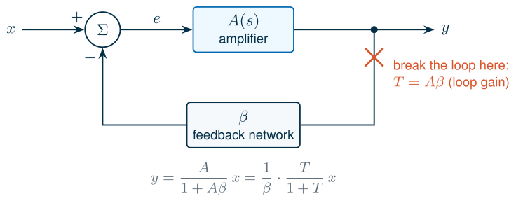
From the figure, \(e = x - \beta y\) and \(y = Ae\), so
\[A_{CL} = \frac{y}{x} = \frac{A}{1+A\beta} = \frac{1}{\beta}\cdot\frac{T}{1+T}, \qquad T = A\beta. \tag{11.1}\]The product \(T\) is the loop gain: the gain a signal sees on one trip around the loop. When \(T \gg 1\), \(A_{CL} \to 1/\beta\), set by the feedback network alone, with a relative error of about \(1/T\). Every benefit of feedback is a division by \(1+T\) [53, 51]:
-
Desensitization. Differentiating Eq. (11.1), a relative change of \(A\) appears in \(A_{CL}\) divided by \(1+T\):
\[\frac{dA_{CL}}{A_{CL}} = \frac{1}{1+T}\cdot\frac{dA}{A}. \tag{11.2}\] - Bandwidth. If \(A\) has a dominant pole at \(\omega_{p1}\), the closed loop has its pole at \(\omega_{p1}(1+T_0)\), where \(T_0\) is the low-frequency loop gain: gain is traded for bandwidth, and the gain-bandwidth product stays the same.
-
Impedance. Feedback that samples the output voltage divides the output resistance by \(1+T\):
\[R_{out,CL} = \frac{R_{out}}{1+T}. \tag{11.3}\] - Linearity. A nonlinear amplifier has a gain that changes with the signal level. Eq. (11.2) applies to those changes too, so the incremental gain of the closed loop varies \(1+T\) times less.
Table 11.1 puts numbers on all four for the amplifier used throughout this chapter: the two-stage Miller OTA that Chapter 12 designs in both PDKs, here connected as a unity-gain follower (\(\beta = 1\), so \(T = A\)) driving 2 pF.
Table 11.1. The four benefits of feedback, simulated: the open-loop OTA against the same OTA as a unity-gain follower.
| Quantity | SG13G2 open loop | SG13G2 follower | SKY130 open loop | SKY130 follower |
|---|---|---|---|---|
| Gain over 5 corners × 3 temperatures | 1100–1430 (±13 %) | error 0.070–0.091 % | 4520–6720 (±20 %) | error 0.015–0.022 % |
| −3 dB bandwidth | 18.7 kHz | 37.6 MHz | 4.0 kHz | 32.2 MHz |
| Output resistance at 1 kHz | 47.8 kΩ | 37 Ω | 94.1 kΩ | 15 Ω |
| Change of incremental gain, \(v_{out}\) from 0.2 V to \(V_{DD}\) − 0.2 V | 48 % | 0.071 % | 68 % | 0.034 % |
The open-loop gain varies by ±13–20 % over process and temperature; the follower’s gain error never exceeds 0.1 %. The bandwidth grows by a factor of about 2000 in SG13G2 and 8000 in SKY130, close to \(1+T_0\). The output resistance falls from tens of kilohms to tens of ohms, exactly as Eq. (11.3) predicts (\(47.8\ \mathrm{k\Omega}/1290 = 37\ \Omega\)). All of this is bought with gain, and paid for with a risk: the loop can oscillate.
11.2 Loop gain
The loop gain is the quantity to compute, measure and design. Conceptually, you break the loop at one point, inject a test signal \(v_t\) into the side that drives the loop, and measure what comes back on the other side, \(v_r\):
\[T = -\frac{v_r}{v_t}\bigg\vert_{x = 0}. \tag{11.4}\]The minus sign makes \(T\) positive at low frequency for negative feedback. The input \(x\) is set to zero (its DC value stays), because the loop gain is a property of the loop, not of the signal. Three facts follow from Eq. (11.1).
- The loop gain, not the amplifier gain, decides accuracy and stability. A follower (\(\beta = 1\)) has the largest loop gain an amplifier can be given, which is why op amps are specified, and tested, as followers: if the follower is stable, every resistive feedback configuration with \(\beta < 1\) is too.
- At the frequency \(f_u\) where \(\lvert T\rvert = 1\), the unity-gain frequency of the loop, the benefits of feedback have run out. Above it the amplifier is effectively open loop.
- The closed loop has a pole wherever \(T(s) = -1\). Whether that can happen is the question of the next section.
Where exactly to break the loop matters in a real circuit, because the injection point has an impedance on each side. We return to this in Section 11.4.
11.3 Stability and phase margin
Imagine a sinusoid travelling around the loop. Negative feedback inverts it once (the minus sign in Eq. (11.4)), and every pole adds a phase lag of up to 90°. If at some frequency the lag reaches 180°, the returned signal is back in phase with the original: the feedback has become positive. If its magnitude is still at least one, the loop sustains an oscillation by itself. The Bode stability criterion, valid for loops whose gain crosses unity once (almost every amplifier), turns this into two numbers read from the Bode plot of \(T\):
Key equation · Phase margin and gain margin
\[\mathrm{PM} = 180^\circ + \angle T(f_u), \qquad \lvert T(f_u)\rvert = 1 \tag{11.5}\] \[\mathrm{GM} = -20\log_{10}\lvert T(f_{180})\rvert, \qquad \angle T(f_{180}) = -180^\circ \tag{11.6}\]The loop is stable when PM > 0 and GM > 0 dB. For good transient behaviour we ask for PM ≥ 60° and GM ≥ 10 dB.
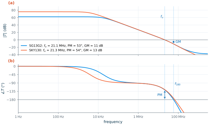
Figure 11.2 shows the loop gain of our two-stage OTA with a plain Miller capacitor, \(C_c\) = 1 pF and no nulling resistor. The dominant pole near 19 kHz (SG13G2) or 4 kHz (SKY130) turns the phase to −90°, and the gain then falls at 20 dB per decade, crossing unity at 21 MHz. Above that, the second pole and the right-half-plane zero (Section 11.7) add lag quickly. At \(f_u\) the phase is −127° in SG13G2, a phase margin of 53°, and the phase reaches −180° at 58 MHz, where the gain is 11 dB below unity. SKY130 behaves almost identically: PM = 54°, GM = 13 dB. Both loops are stable, but by Section 11.5’s standards not by enough.
Common pitfall · Reading the phase margin from the open-loop gain of the wrong circuit
The phase margin belongs to a loop, not to an amplifier. An OTA with 70° in a follower has more margin with \(\beta = 1/10\), because \(\lvert T\rvert = \lvert A\rvert/10\) crosses unity at a lower frequency, where the phase lag is smaller. Conversely, a feedback capacitor at the inverting input, a large load capacitance or the input capacitance of the next stage can all add poles to \(T\) that are not in \(A\). Always measure the loop gain of the circuit you will build, with its real load.
11.4 Measuring loop gain in simulation
Eq. (11.4) says “break the loop”, but a high-gain amplifier cannot be simulated open: with a gain of 1000, its DC operating point needs the input to be correct to a fraction of a millivolt, otherwise the output sits on a rail. The usual way out is the LC break: a huge inductor (say 1 TH) closes the loop at DC, so the bias is right, and opens it at every frequency of interest, while a huge capacitor couples the AC test source into the input side. It is simple and every simulator can do it. It is also subtly wrong whenever the break point is not ideal: the side that drives the loop loses its load (the inductor is an open circuit), and the side that is driven sees an ideal source instead of the real output impedance.
Middlebrook’s double injection
Middlebrook showed in 1975 that the error can be removed exactly [77]. Inject twice at the same point, without opening anything. First a voltage \(v_t\) in series with the loop; measure the voltages on both sides and form \(T_v = -v_o/v_f\), where \(v_o\) is on the side that drives the loop (the amplifier output) and \(v_f\) on the side that feeds back. Then a current \(i_t\) into the node; measure how it splits between the two sides and form \(T_i\) from the two currents. Neither is the loop gain on its own, but together they give it exactly:
Key equation · Loop gain from double injection
\[T = \frac{T_v\,T_i - 1}{T_v + T_i + 2} \tag{11.7}\]\(T_v\) and \(T_i\) are the voltage and current loop gains measured at the same point. Neither injection opens the loop, so the DC bias is unchanged.
Tian, Visvanathan, Hantgan and Kundert turned this into a general simulator probe [78]: a zero-volt voltage source in series with the loop and a zero-ampere current source to ground, inserted at any point of a single loop, with two AC analyses (one per source) and a formula equivalent to Eq. (11.7). This is the method behind the stability analyses of commercial simulators. In ngspice we can do it with two copies of the circuit in one netlist, one per injection, which needs a single AC analysis (Figure 11.3).
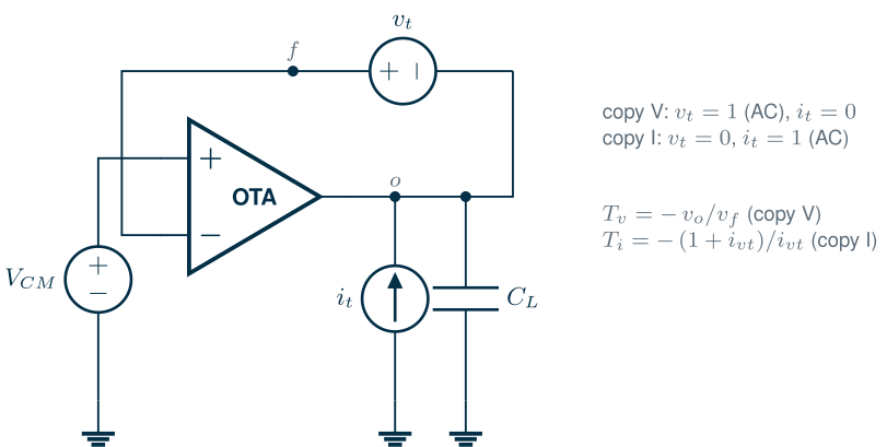
For the current injection, write \(i_{vt}\) for the current that flows from \(f\) through the voltage source to \(o\). The injected 1 A splits into \(1 + i_{vt}\) flowing into the amplifier side and \(-i_{vt}\) into the feedback side, so \(T_i = -(1+i_{vt})/i_{vt}\). The algebra that turns \(T_v\) and \(T_i\) into Eq. (11.7) is short:
Derivation · Why the double injection gives the loop gain
Describe the circuit seen from the break point by its admittances. The amplifier side (node \(o\)) draws a current \(Y_{11}v_o + Y_{12}v_f\); the feedback side (node \(f\)) draws \(Y_{21}v_o + Y_{22}v_f\). In a unilateral loop, \(Y_{21} = 0\) and the return ratio is \(T = Y_{12}/(Y_{11}+Y_{22})\).
Voltage injection: \(v_f - v_o = v_t\) and the same current flows out of one side and into the other: \(Y_{11}v_o + Y_{12}v_f = -(Y_{21}v_o + Y_{22}v_f)\), so \(T_v = -v_o/v_f = (Y_{12}+Y_{22})/(Y_{11}+Y_{21})\).
Current injection: both sides share one voltage \(v\); the currents into them are \((Y_{11}+Y_{12})v\) and \((Y_{21}+Y_{22})v\), so \(T_i = (Y_{11}+Y_{12})/(Y_{21}+Y_{22})\).
Substituting into Eq. (11.7) and simplifying gives, for \(Y_{21}=0\), exactly \(Y_{12}/(Y_{11}+Y_{22})\). In general (bilateral loops) it gives a \(T\) with \(1+T = (Y_{11}+Y_{12}+Y_{21}+Y_{22})/(Y_{11}+Y_{22}+2Y_{21})\), whose zeros are exactly the natural frequencies of the closed loop. We checked our implementation against a behavioural loop whose return ratio is known analytically: the two agree to 1 part in 1012.
The testbench below measures the loop gain of the course OTA (the subcircuit of Chapter 12). Only the model and subcircuit lines differ between the PDKs. The full files, which also run a step response, are tools/figs/ch12_tb_sg13g2.spice and ch12_tb_sky130.spice.
* loop gain of the Chapter 12 OTA, SG13G2 (paths as in IIC-OSIC-TOOLS)
.control
pre_osdi /foss/pdks/ihp-sg13g2/libs.tech/ngspice/osdi/psp103.osdi
.endc
.lib /foss/pdks/ihp-sg13g2/libs.tech/ngspice/models/cornerMOSlv.lib mos_tt
.include ch12_ota_sg13g2.spice
Vdd vdd 0 1.2
Vcm vcm 0 0.6
* copy V: series voltage injection between output ov and feedback node fv
Irefv vdd ibv 10u
Xv vcm fv ov vdd 0 ibv ota2s
CLv ov 0 2p
Vtv fv ov dc 0 ac 1
* copy I: shunt current injection into the output oi
Irefi vdd ibi 10u
Xi vcm fi oi vdd 0 ibi ota2s
CLi oi 0 2p
Vti fi oi dc 0
Iti 0 oi dc 0 ac 1
.control
ac dec 40 1 3e9
let tv = -v(ov)/v(fv)
let ii = i(vti)
let ti = (1 + ii)/(-ii)
let t = (tv*ti - 1)/(tv + ti + 2)
let tdb = db(t)
let tph = 180/pi*cph(t)
meas ac a0_db find tdb at=10
meas ac fu when tdb=0
meas ac ph_fu find tph when tdb=0
let pm = 180 + ph_fu
print pm
.endc
.end
* loop gain of the Chapter 12 OTA, SKY130 (paths as in IIC-OSIC-TOOLS)
.lib /foss/pdks/sky130A/libs.tech/ngspice/sky130.lib.spice tt
.include ch12_ota_sky130.spice
Vdd vdd 0 1.8
Vcm vcm 0 0.9
* copy V: series voltage injection between output ov and feedback node fv
Irefv vdd ibv 10u
Xv vcm fv ov vdd 0 ibv ota2s
CLv ov 0 2p
Vtv fv ov dc 0 ac 1
* copy I: shunt current injection into the output oi
Irefi vdd ibi 10u
Xi vcm fi oi vdd 0 ibi ota2s
CLi oi 0 2p
Vti fi oi dc 0
Iti 0 oi dc 0 ac 1
.control
ac dec 40 1 3e9
let tv = -v(ov)/v(fv)
let ii = i(vti)
let ti = (1 + ii)/(-ii)
let t = (tv*ti - 1)/(tv + ti + 2)
let tdb = db(t)
let tph = 180/pi*cph(t)
meas ac a0_db find tdb at=10
meas ac fu when tdb=0
meas ac ph_fu find tph when tdb=0
let pm = 180 + ph_fu
print pm
.endc
.end
The cph function returns the continuous (unwrapped) phase in radians, and meas finds the crossing (ngspice manual [36]). In IIC-OSIC-TOOLS the testbench prints \(A_0\) = 62.2 dB, \(f_u\) = 21.5 MHz and PM = 67.0° for SG13G2, and 75.7 dB, 21.7 MHz and 72.8° for SKY130.
When the naive break goes wrong
To see the difference, we connect the OTA as a non-inverting amplifier with a gain of 2 (\(R_1 = R_2\) = 10 kΩ, so \(\beta = 1/2\)) and measure its loop gain three ways: with the probe, with an LC break at the OTA output, and with an LC break at the inverting input. Figure 11.4 shows the result.
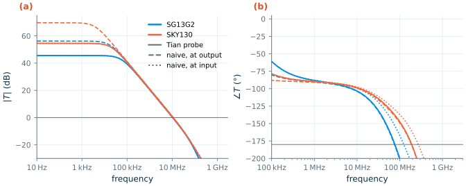
- Break at the output. The OTA’s output resistance is 48 kΩ (SG13G2) and 94 kΩ (SKY130), but the 20 kΩ feedback network that loads it in reality has disappeared behind the inductor. The low-frequency loop gain comes out 10.6 dB too high in SG13G2 (56.2 dB instead of 45.6 dB) and 15.1 dB too high in SKY130 (69.7 instead of 54.5 dB). Because \(f_u\) is set by \(g_{m}/C_c\), not by the output resistance, the phase margin happens to be only 1.3° off here.
- Break at the input. Now the source drives the gate of the input transistor, an almost ideal load, and the low-frequency gain is right. But the feedback network’s tap, a 5 kΩ node, has lost the 0.3 pF gate capacitance of the SG13G2 input pair that loads it in reality. The measured phase margin is 80.1° instead of 76.0° in SG13G2 and 82.0° instead of 80.9° in SKY130, whose input pair is four times smaller.
What this means for your design
A single injection is accurate only where the impedance looking back from the break point is much smaller than the impedance looking forward, Middlebrook’s original condition [77]. Real circuits rarely offer such a point: the output of an OTA is a high-impedance node by design. Use the double-injection probe by default; it costs one extra copy of the circuit and is exact for any single loop. Keep the LC break for quick checks where you know the impedances.
SG13G2 vs SKY130 · The same probe, different model plumbing
The probe uses only ideal sources, so it works unchanged with both PDKs. The difference is in the models: the SG13G2 PSP model is compiled Verilog-A and must be loaded before the netlist is parsed, with
pre_osdior theosdicommands of the IHP PDK’s own.spiceinit[37], while SKY130’s BSIM4 is built into ngspice [19] but needsset ngbehavior=hsain.spiceinitto bin multi-finger devices correctly (Section 12.6). The AC analysis of the two-copy testbench takes about one second in either PDK.
11.5 Two-pole systems and the step response
Why ask for 60° of phase margin when anything above zero is stable? Because the margin decides how the loop responds in time. Most amplifiers behave near \(f_u\) like a loop with one integrator and one more pole \(\omega_{p2}\):
\[T(s) \approx \frac{\omega_u}{s\,(1+s/\omega_{p2})}, \qquad A_{CL}(s) = \frac{T}{1+T} = \frac{\omega_n^2}{s^2 + 2\zeta\omega_n s + \omega_n^2}, \qquad \omega_n = \sqrt{\omega_u\omega_{p2}},\ \ \zeta = \frac{1}{2}\sqrt{\frac{\omega_{p2}}{\omega_u}}. \tag{11.8}\]The closed loop is a second-order system with damping ratio \(\zeta\). The phase margin and the overshoot of the step response both depend only on \(\zeta\) [52, 51]:
\[\mathrm{PM} = \arctan\frac{2\zeta}{\sqrt{\sqrt{1+4\zeta^4}-2\zeta^2}}, \qquad \text{overshoot} = \exp\!\left(\frac{-\pi\zeta}{\sqrt{1-\zeta^2}}\right). \tag{11.9}\]Eliminating \(\zeta\) gives the dashed curve in Figure 11.5b: 45° of phase margin means 23 % overshoot, 60° means 8.8 %, and above about 76° (\(\zeta \ge 1\)) there is none. In terms of the second pole, \(\mathrm{PM} \approx 90^\circ - \arctan(\omega_u/\omega_{p2})\): PM = 60° needs \(\omega_{p2} \approx 1.7\,\omega_u\), PM = 70° needs \(2.7\,\omega_u\).
To test this on a real amplifier, we change the phase margin of the OTA by changing \(C_c\) from 0.15 to 2.2 pF, with \(R_z = 1/g_{m6}\) so that the zero of Section 11.7 is out of the way, and apply a 10 mV step to the follower. Each pair of points in Figure 11.5b is one loop-gain simulation (the PM) and one transient simulation (the overshoot).
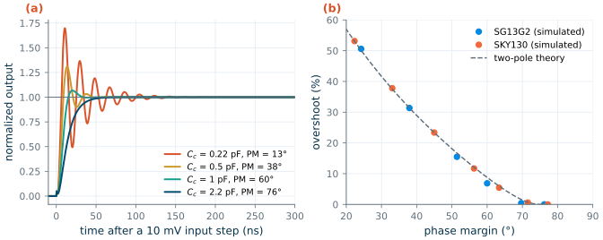
The agreement is remarkable for a circuit with eight transistors: across both PDKs, every point lies within a few percent of the curve. At 60° the SG13G2 follower overshoots by 6.9 %, the theory says 8.8 %, and the small difference comes from the higher poles that Eq. (11.8) ignores. The step responses in panel (a) show the trade-off that makes 60–70° the usual target. Less margin rings and takes long to settle; much more margin means a larger \(C_c\), a lower \(f_u\) and a slower rise. In SG13G2 the follower settles to 1 % in 31 ns with \(C_c\) = 1 pF (PM = 60°) and in 27 ns with 1.5 pF (PM = 70°), which is almost free of overshoot while \(f_u\) is still 15 MHz. With 2.2 pF (PM = 76°) it needs 52 ns, because \(f_u\) has halved, and with 0.5 pF (PM = 38°) the ringing stretches it to 51 ns. SKY130 shows the same optimum.
11.6 Miller compensation and pole splitting
A two-stage amplifier has two high-impedance nodes, the output of each stage, and therefore two low-frequency poles of comparable size. Without compensation both lie in the megahertz range (Figure 11.7a, \(C_c\) = 0.01 pF), and the phase reaches −180° while the gain is still large: unstable in a follower. Miller compensation connects a capacitor \(C_c\) across the second stage. Seen from the first stage, the second stage multiplies it by its gain (the Miller effect of Chapter 9), which makes the first pole very low. At high frequency, \(C_c\) shorts the output to the gate of the second-stage transistor, which then behaves like a diode with a conductance \(g_{m6}\), so the output pole moves up. The two poles split apart.
Figure 11.6 is the small-signal model. \(R_1\), \(C_1\) and \(R_2\), \(C_2\) are the resistance and capacitance at the two nodes; \(R_z\) is the nulling resistor of Section 11.7.
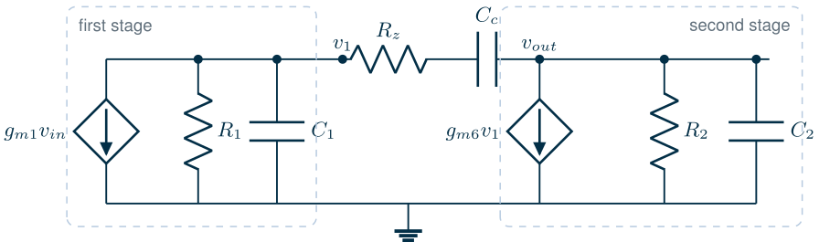
Writing the node equations of Figure 11.6 with \(R_z = 0\) gives the transfer function [53, 54]
\[\frac{v_{out}}{v_{in}} = g_{m1}R_1\,g_{m6}R_2\,\frac{1 - s\,C_c/g_{m6}}{1 + a_1 s + a_2 s^2}, \tag{11.10}\] \[a_1 = R_1(C_1+C_c) + R_2(C_2+C_c) + g_{m6}R_1R_2C_c, \qquad a_2 = R_1R_2\left[C_1C_2 + C_c(C_1+C_2)\right]. \tag{11.11}\]The two poles are the roots of \(1 + a_1 s + a_2 s^2\). When they are far apart, \(p_1 \approx 1/a_1\) and \(p_2 \approx a_1/a_2\), and since the \(g_{m6}R_1R_2C_c\) term dominates \(a_1\):
Key equation · Pole splitting
\[p_1 \approx \frac{1}{g_{m6}R_1R_2\,C_c}, \qquad p_2 \approx \frac{g_{m6}\,C_c}{C_1C_2 + C_c(C_1+C_2)} \xrightarrow{\ C_c \gg C_1\ } \frac{g_{m6}}{C_1 + C_2}, \qquad \omega_u \approx \frac{g_{m1}}{C_c}. \tag{11.12}\]Increasing \(C_c\) lowers \(p_1\) in proportion and raises \(p_2\) until it saturates near \(g_{m6}/C_2\). The unity-gain frequency depends only on \(g_{m1}\) and \(C_c\).
Figure 11.7 shows pole splitting in both PDKs. We sweep \(C_c\) from 0.01 to 2 pF, extract the two lowest poles from each simulated loop gain by fitting a two-pole model below \(3f_u\), and compare them with the roots of Eq. (11.11), evaluated with \(R_1\), \(R_2\), \(C_1\), \(C_2\) and \(g_{m6}\) from the simulated operating point (for SG13G2: 174 kΩ, 48 kΩ, 0.30 pF, 2.03 pF and 1.01 mS).
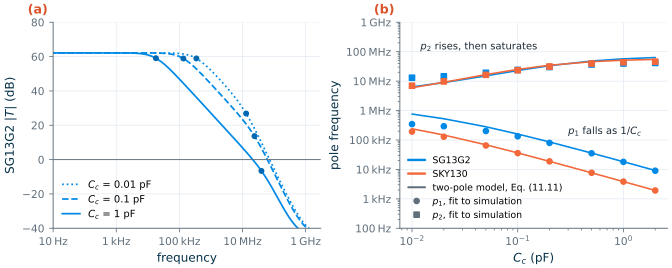
For \(C_c \ge 0.5\) pF the first pole agrees with the model to within 2 %: at 1 pF, 18.2 kHz predicted and 18.0 kHz fitted in SG13G2, 3.85 kHz for both in SKY130. The second pole agrees well up to about 0.2 pF and then falls behind: at 1 pF the model says 57 MHz (SG13G2) and 51 MHz (SKY130), the fit 40 and 44 MHz. The fit is not wrong; it lumps into “\(p_2\)” the other poles of the real circuit, the mirror pole near 220 MHz and the pole of \(R_z\) with \(C_1\), which also add phase lag near \(f_u\). For very small \(C_c\) the model’s first pole is too high (760 kHz against 345 kHz at 0.01 pF): the gate-drain capacitance of \(M_6\), about 40 fF in SG13G2, is a Miller capacitor that is always there, and Eq. (11.11) does not include it.
Worked example 11.1 · Choosing Cc for 60° in SG13G2
Hand estimate. We want \(f_u\) near 21 MHz and PM = 60°, so \(f_{p2} \ge 1.7 f_u\) = 36 MHz. With \(g_{m6}\) = 1.01 mS, \(C_1\) = 0.30 pF and \(C_2\) = 2.03 pF, Eq. (11.12) gives \(f_{p2}\) = 36 MHz already at \(C_c \approx\) 0.3 pF; we take 1 pF to keep \(f_u\) near 21 MHz, which gives \(f_{p2}\) = 57 MHz (exact roots of Eq. (11.11)). At \(C_c\) = 1 pF the estimate is \(\mathrm{PM} = 90^\circ - \arctan(21/57) = 70^\circ\).
Simulation. At \(C_c\) = 1 pF the simulated phase margin is 60.0° in SG13G2 and 63.4° in SKY130 (with \(R_z = 1/g_{m6}\)). The hand estimate is 10° optimistic, the same discrepancy as in Figure 11.7: the mirror pole and the \(R_zC_1\) pole together cost about 10° at 21 MHz. Use the two-pole formula to choose the starting point and the loop-gain simulation to decide.
11.7 The right-half-plane zero
Eq. (11.10) has a zero at \(s = +g_{m6}/C_c\), in the right half of the s-plane. Physically, \(C_c\) is a second path from \(x_1\) to the output: at high frequency it carries a current \(sC_cv_1\) forward, while \(M_6\) pulls \(g_{m6}v_1\) in the opposite direction. At \(\omega = g_{m6}/C_c\) the two cancel and the output does not respond. A right-half-plane zero is the worst of both worlds: it raises the gain like a left-half-plane zero but lags the phase like a pole. Because \(C_c\) is large and \(g_{m6}\) modest in a low-power design, the zero sits close to \(p_2\): here \(g_{m6}/(2\pi C_c)\) = 160 MHz in SG13G2, less than eight times \(f_u\), costing about 8° of phase margin.
The cure is to make the feedforward path one-way. A resistor \(R_z\) in series with \(C_c\) moves the zero to
Key equation · Zero of the compensation branch
\[f_z = \frac{1}{2\pi C_c\,(1/g_{m6} - R_z)}. \tag{11.13}\]\(R_z = 0\): right-half-plane zero at \(g_{m6}/(2\pi C_c)\). \(R_z = 1/g_{m6}\): zero at infinity. \(R_z > 1/g_{m6}\): left-half-plane zero, which adds phase lead. \(R_z = (1+C_2/C_c)/g_{m6}\) places it on top of \(p_2\) and cancels it.
The resistor adds a third pole, at roughly \(1/(2\pi R_zC_1)\), which must stay well above \(f_u\); with \(C_1\) = 0.3 pF and \(R_z\) = 2 kΩ it sits near 260 MHz. Figure 11.8 shows the effect in both PDKs, with \(C_c\) = 1 pF.
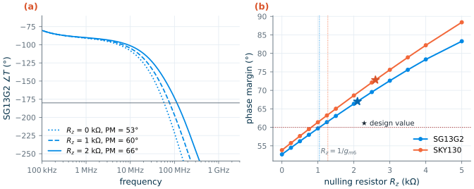
Without \(R_z\) the phase margin is 53° (SG13G2) and 54° (SKY130). Moving the zero to infinity with \(R_z = 1/g_{m6}\) (1.04 kΩ and 1.28 kΩ) restores 60° and 63°: the right-half-plane zero was costing 7–10°, close to the estimate above. Beyond that the zero moves into the left half-plane and the margin keeps rising, to 67° and 73° at the design values of 2.1 and 2.6 kΩ, and above 80° at 5 kΩ. More is not always better. The gain margin peaks at about 2–2.5 kΩ (18 dB and 29 dB) and then falls, because the third pole moves down as \(R_z\) grows; and a left-half-plane zero that lands near or below \(f_u\) forms a pole–zero doublet with \(p_2\), whose slow tail lengthens settling. The design values, halfway between \(1/g_{m6}\) and full cancellation of \(p_2\), are a robust middle: the zero lies at several times \(f_u\), and the margin changes slowly if \(g_{m6}\) or \(R_z\) drift.
Common pitfall · A nulling resistor that does not track
Eq. (11.13) compares a resistor with \(1/g_{m6}\), a transconductance. Over corners and temperature a poly resistor moves by ±10–20 %, and \(g_{m6}\) moves differently. Designs that rely on exact cancellation (\(R_z = (1+C_2/C_c)/g_{m6}\)) lose it at the corners and leave a doublet behind. Two defences: choose \(R_z\) in the flat part of Figure 11.8b, as Chapter 12 does, or replace it by a MOS transistor in triode biased from the same mirror as \(M_6\), whose on-resistance tracks \(1/g_{m6}\) [54, 51]. Check the phase margin at all corners either way (Section 12.8).
Try it · Lab 6
In Lab 6 you build the probe testbench of Figure 11.3 around your OTA, sweep \(C_c\) and \(R_z\), and reproduce Figures 11.5 and 11.8 for your PDK. Then replace the probe by an LC break at the output and at the input, as in Figure 11.4, and explain the differences.
- Negative feedback divides every imperfection by \(1+T\): in our OTA it turns ±13–20 % of gain variation into less than 0.1 % of error, and 48 kΩ of output resistance into 37 Ω.
- Stability is read from the loop gain \(T\): the phase margin at \(f_u\) and the gain margin at \(f_{180}\). Test op amps as followers, the configuration with the largest loop gain.
- Measure \(T\) without opening the loop: Middlebrook’s double injection, packaged as Tian’s probe, is exact for any single loop and takes one extra circuit copy in ngspice. A naive LC break can be wrong by 10–15 dB of gain or several degrees of phase.
- Phase margin predicts the step response: 45° gives 23 % overshoot, 60° about 8 %, and the simulated OTAs follow the two-pole theory closely.
- Miller compensation splits the poles: \(p_1 \propto 1/C_c\), \(p_2 \to g_{m6}/C_2\), \(\omega_u = g_{m1}/C_c\). Its right-half-plane zero costs 7–10° here; a nulling resistor \(R_z \ge 1/g_{m6}\) removes it and, set a little higher, adds phase lead.
Further reading
- R. D. Middlebrook [77]: the original double-injection paper, still the clearest account of why single injection fails.
- M. Tian, V. Visvanathan, J. Hantgan and K. Kundert [78]: loop-based and device-based stability analysis in a simulator.
- P. R. Gray, P. J. Hurst, S. H. Lewis and R. G. Meyer [53]: feedback, frequency response and compensation of the two-stage op amp in depth.
- T. Chan Carusone, D. A. Johns and K. W. Martin [52]: a compact treatment of second-order loops, phase margin and settling.
- B. Razavi, Design of Analog CMOS Integrated Circuits [51]: stability and frequency compensation, including other compensation schemes.