Chapter 1
Why RF, Why Open Source
A radio chip hears a signal of a few microvolts at its antenna and answers with a volt, at gigahertz frequencies, from a supply of about one volt. This chapter shows where radios live in the spectrum, what makes designing for them different from the analog design you already know, which silicon is good at it, and the open-source tools and the two projects, a 2.4 GHz transceiver and a 50 GHz amplifier, that the rest of the course builds on.
- Place common wireless systems in the radio spectrum and convert between frequency and wavelength.
- Work with power in dBm at 50 Ω interfaces, and decide when a wire must be treated as a transmission line.
- Name the blocks of a transceiver and the trade-offs between noise, linearity, gain, frequency, power and supply voltage.
- Compare CMOS, SiGe BiCMOS and III–V technologies for RF, and describe the RF devices and metal stack of IHP SG13G2.
- Describe the open-source RF design flow, and state the specifications of the course radio and of the 50 GHz amplifier.
Contents
- 1.1 Radio in every pocket: wireless systems and the spectrum
- 1.2 What makes RF design different
- 1.3 The anatomy of a transceiver
- 1.4 Silicon for RF: CMOS, SiGe BiCMOS and IHP SG13G2
- 1.5 The open-source RF flow
- 1.6 The course radio: a 2.4 GHz transceiver and a 50 GHz amplifier
- 1.7 How to use this course
- Further reading
1.1 Radio in every pocket: wireless systems and the spectrum
A smartphone carries half a dozen radios: cellular, Wi-Fi, Bluetooth, satellite navigation (GNSS), near-field communication (NFC) and, in recent models, ultra-wideband (UWB) ranging. A watch, a car key or a wireless earbud carries at least one. Each of these radios transmits and receives in its own slice of the electromagnetic spectrum, allocated by the International Telecommunication Union’s Radio Regulations and by national regulators [181]. Radio frequency (RF) design is the design of the circuits that generate, amplify, filter and convert these signals.
A wave of frequency \(f\) travelling at the speed of light \(c\) has a free-space wavelength
\[\lambda_0 = \frac{c}{f}. \tag{1.1}\]Figure 1.1 places common systems on a logarithmic frequency axis, with the wavelength on top. The ITU names the decades of frequency: VHF (30–300 MHz), UHF (0.3–3 GHz), SHF (3–30 GHz) and EHF (30–300 GHz), the millimetre-wave band, where \(\lambda_0\) is between 10 and 1 mm [181]. Microwave engineers more often use the IEEE radar letter bands [182]: the course radio at 2.44 GHz sits in S band (2–4 GHz) and the 50 GHz amplifier of Chapter 17 in V band (40–75 GHz).
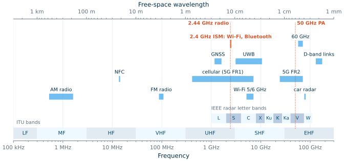
Why have radios climbed from the megahertz of AM broadcasting to tens of gigahertz? Two reasons. First, bandwidth: a band a few per cent wide holds far more hertz, and so more bits per second, at 30 GHz than at 300 MHz; the 5G millimetre-wave bands (FR2, 24.25–71 GHz) offer channels hundreds of megahertz wide [183]. Second, antennas: a half-wave dipole is 61.4 mm long at 2.44 GHz but only 3.0 mm at 50 GHz, small enough for an array of antennas on a package. The price is paid in the circuits: transistors have less gain at higher frequencies (Section 1.4), and every wire becomes a transmission line (Section 1.2).
The course radio works in the 2.4 GHz ISM band. The ITU designates 2400–2500 MHz for industrial, scientific and medical (ISM) equipment, such as microwave ovens, worldwide [181]; national rules let licence-free radios use 2.400–2.4835 GHz of it, under limits on their transmitted power. Wi-Fi [186] and Bluetooth [184] share this band, which is why it is crowded, and why a receiver for it must tolerate strong interferers.
1.2 What makes RF design different
An analog designer thinks in voltages and currents: a gain in V/V, an output swing, a bandwidth. An RF designer thinks in power and impedance, and in a frequency range where the wavelength approaches the size of the circuit. Four ideas follow.
Power, not voltage
Between chips, an RF signal travels through cables, connectors, filters, printed-circuit traces and antennas, all designed for one characteristic impedance \(Z_0\), the ratio of voltage to current in a travelling wave (Chapter 3). When every block presents \(Z_0\) at its ports, a source delivers its available power, the most it can deliver, to the next block, and nothing is reflected. Power is then the quantity that flows through the chain, so RF engineers specify gains as power gains in decibels and signal levels in dBm, decibels relative to one milliwatt:
\[P_{dBm} = 10\log_{10}\frac{P}{1\ \mathrm{mW}}. \tag{1.2}\]A sinusoid of peak amplitude \(V_p\) in a resistance \(R\) carries
\[P = \frac{V_p^2}{2R} = \frac{V_{rms}^2}{R}, \tag{1.3}\]so 0 dBm in 50 Ω is a sinusoid of 0.316 V peak. The other reference every RF designer knows by heart is the thermal noise of a resistor at \(T_0\) = 290 K, which delivers \(kT_0\) to a matched load in each hertz of bandwidth \(B\) [6]:
\[P_n = kT_0B \;\Rightarrow\; P_{n,dBm} = -174\ \mathrm{dBm/Hz} + 10\log_{10}\frac{B}{1\ \mathrm{Hz}}. \tag{1.4}\]Worked example 1.1 · The dynamic range of the course radio
The receiver of the course radio (Section 1.6) must work with −90 dBm at its antenna, and its transmitter delivers +10 dBm. In 50 Ω, Eq. (1.3) turns these into voltages:
- receiver sensitivity, −90 dBm = 1.0 pW: \(V_p = \sqrt{2\cdot 50\ \Omega\cdot 1.0\ \mathrm{pW}}\) = 10.0 µV, or 7.07 µV rms;
- transmitter output, +10 dBm = 10 mW: \(V_p = \sqrt{2\cdot 50\ \Omega\cdot 10\ \mathrm{mW}}\) = 1.00 V, or 0.707 V rms.
The two differ by 100 dB in power, a factor of 100 000 in voltage. By Eq. (1.4) the noise in the radio’s 1 MHz bandwidth is −173.98 + 60 ≈ −114 dBm, so the weakest wanted signal is only 24 dB above the noise of an ideal 50 Ω source; the receiver may add only a few decibels of noise of its own (Chapter 4). At the other end, 1.00 V peak is most of the 1.2 V supply of SG13G2’s core transistors: the power amplifier will need an impedance transformation, or a higher supply, to deliver it (Chapter 16).
Common pitfall · 20 log is not always the power gain
A voltage gain \(A_v\) expressed as \(20\log_{10}\vert A_v\vert\) equals the power gain in dB only when the input and output resistances are equal. In general the power gain is \(A_v^2R_{in}/R_L\): an LNA with a 50 Ω input that drives the 2 kΩ input of a mixer with 20 dB of voltage gain has a power gain of only 4.0 dB. Say which gain you mean, and with dBm always say into which impedance.
Why 50 Ω
Why 50 Ω, and not 75 or 100? One explanation lies in the coaxial cable. For an air-filled line with inner and outer conductor radii \(a\) and \(b\), the conductor loss for a given outer diameter is lowest at \(b/a\) = 3.59, a characteristic impedance of 76.7 Ω, while the power the line can carry before the air breaks down is highest at \(b/a\) = 1.65, or 30.0 Ω [8]. 50 Ω lies between the two (their geometric mean is 48.0 Ω), and became the standard for cables, connectors, filters and test equipment. Inside a chip nothing needs to be 50 Ω; only the interfaces to the outside world, the antenna, the off-chip filters and the measurement equipment, do. Getting from one to the other is the job of the matching networks of Chapter 8.
Derivation · The two optimum coaxial impedances
An air-filled coaxial line has \(Z_0 = (\eta_0/2\pi)\ln(b/a) = 60\ \Omega\cdot\ln x\), with \(x = b/a\). Its conductor loss per metre is proportional to \((1/a + 1/b)/\ln x\) [8]; for a fixed outer radius \(b\) this is proportional to \((1 + x)/\ln x\), which is smallest at \(x\) = 3.59, \(Z_0\) = 76.7 Ω. The field is strongest at the inner conductor, \(E_{max} = V/(a\ln x)\), so for a fixed breakdown field the largest voltage is \(V = E_{max}\,a\ln x\) and the power \(V^2/(2Z_0)\) is proportional to \(a^2\ln x\), or, for a fixed \(b\), to \(\ln x/x^2\). That is largest at \(x = \sqrt{e}\) = 1.65, \(Z_0\) = 30.0 Ω. The script of this chapter finds both optima numerically.
Distributed effects
A wire is a lumped element, with the same current along its whole length at any instant, only while it is short compared with the wavelength. On a chip, the wave travels in silicon dioxide, of relative permittivity \(\varepsilon_r\) = 4.1 in SG13G2 [200], so it is slower and its wavelength shorter than in free space:
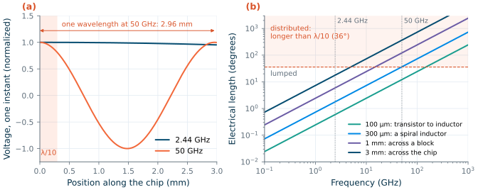
\[\lambda = \frac{c}{f\sqrt{\varepsilon_r}}, \qquad \theta = 360°\,\frac{\ell}{\lambda}. \tag{1.5}\]The electrical length \(\theta\) of a line of length \(\ell\) is the phase a wave accumulates along it. A common rule treats a line as lumped below \(\lambda/10\), or 36°, and as a distributed element, a transmission line, above [8]. (A line with air above it has a slightly longer wavelength, so Eq. (1.5) with \(\varepsilon_r\) = 4.1 is a little pessimistic.)
Worked example 1.2 · How long is a wire?
On chip, Eq. (1.5) gives \(\lambda\) = 60.7 mm at 2.44 GHz and 2.96 mm at 50 GHz, so \(\lambda/10\) is 6.07 mm and 0.296 mm. Figure 1.2b reads off the electrical lengths at 2.44 and at 50 GHz, and the frequency at which each wire reaches λ/10:
- 100 µm, from a transistor to an inductor: 0.59° and 12.2°; λ/10 at 148 GHz;
- 300 µm, across a spiral inductor: 1.78° and 36.5°; λ/10 at 49.4 GHz;
- 1 mm, across a block: 5.93° and 122°; λ/10 at 14.8 GHz;
- 3 mm, across the chip: 17.8° and 365°; λ/10 at 4.94 GHz.
At 2.44 GHz every on-chip wire is lumped, and the course radio can be designed with inductors, capacitors and resistors; the bond wires, the package and the board traces to the antenna, millimetres to centimetres long, are not. At 50 GHz any wire longer than about 0.3 mm is a transmission line, and the matching networks of the amplifier are built from lines (Chapter 17).
The RF design hexagon
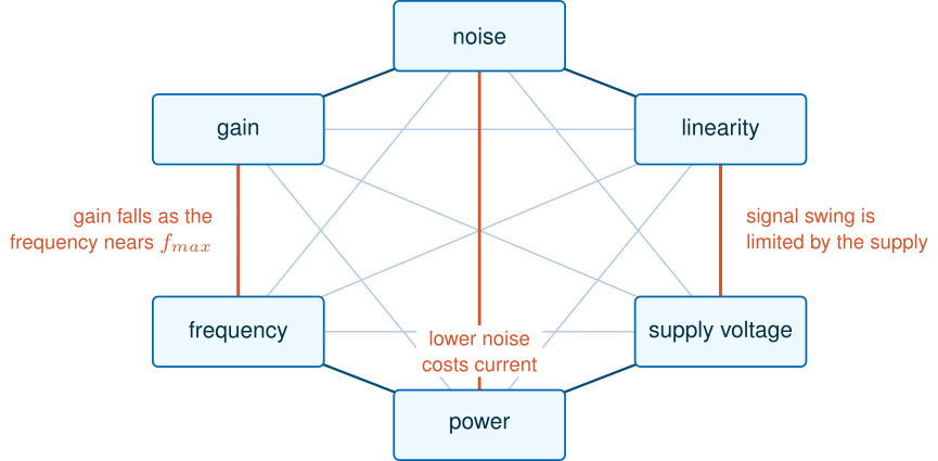
Analog design is a game of trade-offs, between gain, speed, noise, swing and power (The Art of Analog IC Design, Chapter 6). Razavi draws the RF version as a hexagon [6]: noise, linearity, gain, frequency, power and supply voltage, each of which can be improved only at the expense of others (Figure 1.3). A low-noise amplifier lowers its noise by spending current (Chapter 9). A large signal must fit between the supply rails, so linearity suffers as supplies shrink (Chapter 4). And a transistor’s power gain falls with frequency until it reaches unity at its \(f_{max}\) (Section 1.4). What makes RF hard is that a radio pushes on all six corners at once.
1.3 The anatomy of a transceiver
Figure 1.4 shows the blocks of a transceiver, a radio that both receives and transmits, drawn as the course radio. The grey labels give the chapters that design each block; Chapter 5 explains why the architecture looks the way it does.
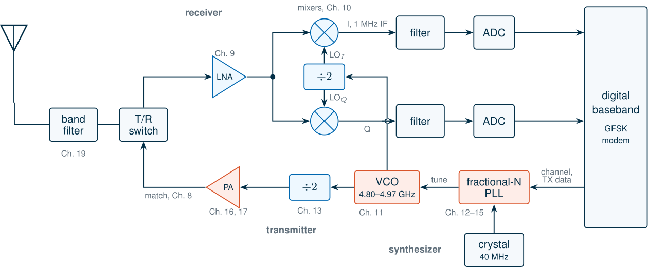
Receiving. The antenna’s signal passes a band filter, which removes strong signals outside the ISM band, and a T/R switch, which connects the antenna to the receiver or the transmitter: a Bluetooth Low Energy radio never does both at once. The low-noise amplifier (LNA) comes first because, by the Friis formula of Chapter 4, the noise of the first stage dominates the noise of the whole receiver. Two mixers multiply the amplified signal by two copies of a local oscillator (LO) signal, 90° apart, and move the wanted channel to an intermediate frequency (IF) of about 1 MHz, as an in-phase (I) and a quadrature (Q) signal (Chapter 10). At 1 MHz, ordinary analog circuits take over: filters that reject the neighbouring channels and analog-to-digital converters (ADCs), the subject of the sibling course (Chapters 19–22); a digital modem then demodulates the bits.
The synthesizer. The LO must step to any of the 40 channels with the accuracy of a crystal oscillator. A voltage-controlled oscillator (VCO) at twice the LO frequency (Chapter 11) feeds a divide-by-two that produces the I and Q phases (Chapter 13), and a phase-locked loop (PLL) locks the VCO to a 40 MHz crystal. With a 1 MHz IF on either side of the 40 channels, the VCO must cover 4.802 to 4.962 GHz (the specified 4.80–4.97 GHz leaves a margin), 120.05 to 124.05 times the crystal frequency, and the channels are 4 MHz apart at the VCO, a tenth of the reference: the division ratio must take fractional values, which is the job of the fractional-N synthesizer of Part IV (Chapters 12–15).
Transmitting. Bluetooth Low Energy uses Gaussian frequency-shift keying (GFSK), a constant-envelope modulation that carries the data in the frequency alone. A common way to transmit it, one of the options Chapter 5 compares, is to modulate the synthesizer itself, divide its output by two, and drive the power amplifier (PA) (Chapter 16). The PA’s output network matches it to the 50 Ω antenna port and also filters its harmonics, at 4.88 and 7.32 GHz.
Of all these blocks, the LNA, the mixers, the VCO, the dividers and the PA work at the carrier frequency or at twice it. They are the subject of this course; the rest is analog or digital design at megahertz frequencies.
Follow a packet through the receiver. The demo below takes a Bluetooth packet from the antenna to bits through the receiver this course designs, with the gains, noise figures, phase noise and I/Q balance that later chapters simulate and Chapter 19 assembles. Step through the five stages, change the signal level, and switch on a strong signal 3 MHz away, a blocker: with the designed synthesizer the receiver keeps enough SNR, but with one 20 dB noisier the blocker’s reciprocal mixing buries the wanted signal. Every term in it is explained in the chapters it links to.
1.4 Silicon for RF: CMOS, SiGe BiCMOS and IHP SG13G2
Three families of technology
Three families of semiconductor technology make radio chips (Table 1.1). CMOS won the mass market: a radio in the same process as the digital modem costs little and needs no second chip, and since the early 2000s whole transceivers have been built in it [24]. Its weaknesses are its low supply voltage, the resistance of its thin polysilicon gates, its lossy substrate, and back-end metal stacks optimized for dense digital wiring rather than for inductors.
SiGe BiCMOS adds a heterojunction bipolar transistor (HBT) to a CMOS process. Germanium in the thin base of the npn transistor creates a built-in field that speeds the electrons across it, giving transit frequencies of hundreds of gigahertz with the lithography of a 130 nm CMOS process [25]. A bipolar transistor also has a large transconductance for its current, \(g_m = I_C/V_T\), low flicker noise, and variants with higher breakdown voltages. IHP’s research HBTs reach an \(f_T\) of 505 GHz and an \(f_{max}\) of 720 GHz [26, 27]. SiGe dominates where performance at high frequency matters more than digital density: automotive radar, optical links and millimetre-wave front ends.
III–V compounds (GaAs, GaN, InP) have the fastest and most robust transistors: InP HBTs exceed 1 THz in \(f_{max}\) [28], and GaN transistors withstand far higher voltages and powers than silicon. But they offer no dense CMOS logic, so they appear as separate chips, typically the power amplifiers and switches of a front-end module.
Table 1.1. Technologies for RF circuits, in broad strokes [24, 25, 28, 10].
| CMOS | SiGe BiCMOS | III–V (GaAs, GaN, InP) | |
|---|---|---|---|
| Fastest transistor | MOSFET, improves with every node | SiGe HBT, fastest in silicon | InP HBT, fastest of all |
| Digital integration | complete systems on chip | CMOS logic of an older node | none |
| Breakdown voltage | low (about the supply) | low for the fastest HBTs, higher for slower variants | high, especially GaN |
| Typical use | transceivers for Wi-Fi, Bluetooth, cellular | radar, millimetre-wave and optical front ends | power amplifiers, switches, front-end modules |
The RF devices of SG13G2
IHP SG13G2 is a 130 nm SiGe:C BiCMOS process with an open PDK [191, 200]. It offers both families of silicon transistor on one chip, and the passive devices a radio needs (Table 1.2).
Table 1.2. The RF toolkit of SG13G2, from IHP's process specification [200] (fT, fmax: four emitters, VCE = 1.2 V, extrapolated from 40 GHz) and the model files [191].
| Device | Name in the PDK | Key numbers |
|---|---|---|
| High-speed SiGe HBT | npn13G2 |
emitter 0.07 × 0.9 µm² per finger; fT 300–350 GHz, fmax 400–450 GHz; BVCEO 1.4–1.6 V, BVCBO 3.8–4.8 V |
| Long-emitter HBT | npn13G2l |
fT 280–330 GHz, fmax 380–430 GHz |
| Higher-voltage HBT | npn13G2v |
fT 90–120 GHz, fmax 280–330 GHz; BVCEO 2.2–2.5 V |
| 1.2 V MOSFETs | sg13_lv_nmos, sg13_lv_pmos |
2.45–2.65 nm oxide, L ≥ 0.13 µm; rfmode=1 adds the gate resistance and non-quasi-static model (PSP 103) |
| 3.3 V MOSFETs | sg13_hv_nmos, sg13_hv_pmos |
7.3–7.5 nm oxide |
| MIM capacitor | cap_cmim, cap_rfcmim |
1.5 fF/µm²; cap_rfcmim models its RF parasitics |
| Varactor | sg13_hv_svaricap |
about 23–40 fF/µm² over its tuning range, Q of 43–62 at 15.8 GHz |
| Resistors | rsil, rppd, rhigh |
7, 260 and 1360 Ω/□ |
| Thick top metals | TopMetal1, TopMetal2 | 2 µm and 3 µm of aluminium, 18 and 11 mΩ/□ |
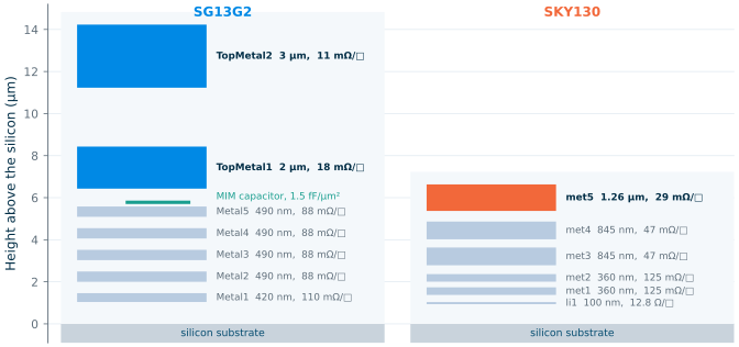
The thick top metals matter as much as the transistors. Figure 1.5 draws the two open back ends to scale. TopMetal2 is 3 µm thick and sits 11.23 µm above the silicon, 2.1 times higher than SKY130’s top metal, met5, at 5.37 µm; its sheet resistance is 2.6 times lower (11 against 29 mΩ/□), so a 1 mm long, 10 µm wide line has 1.1 Ω of resistance in SG13G2 and 2.9 Ω in SKY130 (at DC; at gigahertz frequencies the skin effect adds more). Lower resistance and less capacitance to the lossy 50 Ω·cm substrate mean spiral inductors of higher quality factor and transmission lines of lower loss (Chapter 7).
Gain at 2.44 and 50 GHz: a first look
How much faster is the HBT than the MOSFETs in practice? A transistor amplifies power only up to a certain frequency, and the best power gain it can give at a frequency, with both ports matched, is a single number that does not depend on the circuit around it. For a two-port that is unconditionally stable (Rollett factor \(K > 1\), Chapter 3) it is the maximum available gain (MAG); for a potentially unstable one (\(K < 1\)), it is the maximum stable gain (MSG), the gain left after just enough loss is added to stabilize it [9]:
Key equation · Maximum stable and maximum available gain
\[\mathrm{MSG} = \left\vert\frac{S_{21}}{S_{12}}\right\vert, \qquad \mathrm{MAG} = \mathrm{MSG}\,\left(K - \sqrt{K^2 - 1}\right)\ \ (K > 1). \tag{1.6}\]We write \(G_{max}\) for whichever applies. It falls with frequency and reaches 0 dB at \(f_{max}\).
Two related figures of merit describe the device itself: the transit frequency \(f_T\), at which the short-circuit current gain \(\vert h_{21}\vert\) falls to one, and the maximum oscillation frequency \(f_{max}\), at which Mason’s unilateral gain \(U\) falls to one. Both gains fall at about 20 dB per decade, so IHP’s process control measures them at 40 GHz and extrapolates [200]:
\[f_T \approx f\,\vert h_{21}(f)\vert, \qquad f_{max} \approx f\,\sqrt{U(f)}. \tag{1.7}\]Chapter 6 studies both in depth. Here we simulate three devices with ngspice’s S-parameter analysis (Chapter 2), each in common source or common emitter, biased through ideal bias tees:
- an SG13G2
sg13_lv_nmoswithrfmode=1, W = 20 µm in ten 2 µm fingers, L = 0.13 µm, at VDS = 1.2 V; - an SG13G2
npn13G2with four emitters (the device of IHP’s specification) at VCE = 1.2 V; - a SKY130
nfet_01v8, W = 20 µm in ten fingers, L = 0.15 µm, at VDS = 1.8 V.
The MOSFETs are biased at 0.2 mA/µm, near the current density at which the \(f_{max}\) of n-MOSFETs peaks in most CMOS generations [29]; in our bias sweep the SG13G2 nMOS reaches 97 % of its peak \(f_{max}\) there. The HBT is biased at the peak of its \(f_T\), found in the same sweep. Because MAG and MSG are ratios of the device’s own parameters, they do not change when a device is made wider or given more emitters at the same current density.
* SG13G2 test bench (.lib cornerHBT.lib hbt_typ, .lib cornerMOSlv.lib mos_tt)
vgg gg 0 dc 0.9397             ; VBE at peak fT (0.9345 V for the nMOS)
lg  gg g 1m                    ; ideal bias tee: L feeds DC ...
cg  p1 g 1m                    ; ... C passes RF
v1  p1 0 dc 0 ac 1 portnum 1 z0 50
vdd dd 0 dc 1.2
ld  dd d 1m
cd  p2 d 1m
v2  p2 0 dc 0 ac 1 portnum 2 z0 50
XQ1 d g 0 0 npn13G2 Nx=4
* XM1 d g 0 0 sg13_lv_nmos W=20u L=0.13u ng=10 m=1 rfmode=1
.control
sp dec 40 1e8 1e12
.endc
* SKY130 test bench: same bias tees and ports, VGS = 1.2 V, VDS = 1.8 V
XM1 d g 0 0 sky130_fd_pr__nfet_01v8 W=20 L=0.15 nf=10 ...
* the model has no gate resistance; a second run adds the 5.36 ohm of the poly fingers:
* rgext g gi 5.36
* XM1 d gi 0 0 sky130_fd_pr__nfet_01v8 W=20 L=0.15 nf=10 ...
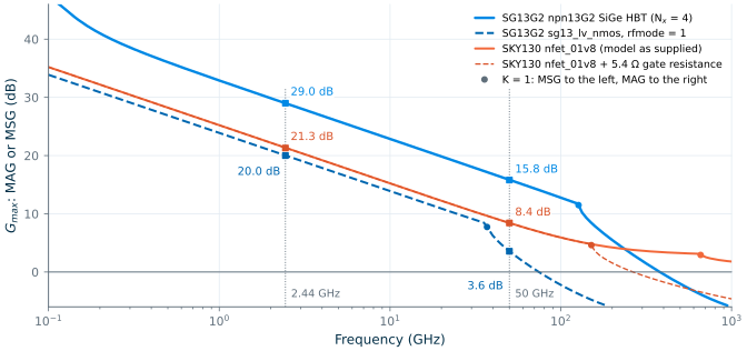
sp analyses: SG13G2 npn13G2 (Nx = 4, VCE = 1.2 V, IC = 10.8 mA), SG13G2 nMOS with rfmode = 1 and SKY130 nfet_01v8 (both W = 20 µm, 0.2 mA/µm, VDS = VDD), tt, 27 °C. Dashed orange: SKY130 with the 5.4 Ω gate resistance its model leaves out. Squares: values at 2.44 and 50 GHz; dots: K = 1.Figure 1.6 and Table 1.3 show the result. At low frequencies all three devices are potentially unstable (\(K < 1\)) and \(G_{max}\) is the MSG, which falls at 10 dB per decade because \(\vert S_{21}/S_{12}\vert\) is roughly \(g_m/(\omega C_{gd})\). At 2.44 GHz the HBT offers 29.0 dB, the SG13G2 nMOS 20.0 dB and the SKY130 nMOS 21.3 dB: all three are good enough for the course radio, which is why its receiver can use the 1.2 V CMOS devices. At 50 GHz the picture changes. The SG13G2 nMOS has crossed \(K\) = 1 at 37 GHz and has only 3.6 dB of MAG left, falling to 0 dB at 74.4 GHz; a single stage would barely amplify, and the loss of any matching network would eat what remains. The HBT still has 15.8 dB, 12.0 dB more. This is why the 50 GHz amplifier of Chapter 17 uses the HBTs.
The HBT’s simulated \(f_T\) of 353 GHz and \(f_{max}\) of 456 GHz, extrapolated from 40 GHz as IHP does it, reproduce the specified 300–350 and 400–450 GHz [200]. Above about 100 GHz the model’s gains no longer fall at exactly 20 dB per decade: \(G_{max}\) reaches 0 dB at 380 GHz, not at 456 GHz. IHP’s process control measures these devices at 40 GHz; read the curves far above that as extrapolations of the model, not as predictions.
Table 1.3. Three transistors compared (simulated, tt, 27 °C; fT and fmax by Eq. 1.7 at 40 GHz).
| SG13G2 nMOS, rfmode = 1 | SG13G2 npn13G2 | SKY130 nfet_01v8 | |
|---|---|---|---|
| Size | W = 20 µm (10 × 2 µm), L = 0.13 µm | Nx = 4 (4 × 0.07 × 0.9 µm²) | W = 20 µm (10 × 2 µm), L = 0.15 µm |
| Bias | VGS = 0.93 V, VDS = 1.2 V | VBE = 0.94 V, VCE = 1.2 V | VGS = 1.20 V, VDS = 1.8 V |
| Current | 4.0 mA (0.2 mA/µm) | 10.8 mA (42.9 mA/µm²) | 4.0 mA (0.2 mA/µm) |
| fT | 80.8 GHz | 353 GHz | 63.5 GHz |
| fmax | 74.3 GHz | 456 GHz | not defined by the model; 286 GHz with 5.4 Ω gate resistance |
| Gmax at 2.44 GHz | 20.0 dB (MSG) | 29.0 dB (MSG) | 21.3 dB (MSG) |
| Gmax at 50 GHz | 3.6 dB (MAG) | 15.8 dB (MSG) | 8.4 dB (MSG) |
| K = 1 at | 37 GHz | 127 GHz | 659 GHz (151 GHz with gate resistance) |
| Gmax = 0 dB at | 74.4 GHz | 380 GHz | above 1 THz (264 GHz with gate resistance) |
SG13G2 vs SKY130 · A model is only as good as its parasitics
SKY130’s nMOS appears to beat SG13G2’s at 50 GHz (8.4 against 3.6 dB), although its \(f_T\) is lower (63.5 against 80.8 GHz). Do not believe it. The SKY130
nfet_01v8model is a BSIM4 model without RF extensions: its gate resistance is switched off (rgatemod = 0). Its input is then almost lossless, Mason’s \(U\) is still 16.2 dB at 100 GHz and never falls to one below 1 THz, and \(f_{max}\) is undefined. The ten 2 µm poly fingers of our device, contacted at both ends, have a gate resistance of \(R_\square W_f/(12\,L\,n_f)\) = 5.36 Ω with SKY130’s 48.2 Ω/□ poly [201]. Adding it gives an \(f_{max}\) of 286 GHz, still 3.8 times that of the SG13G2 device, whoserfmode=1model includes the gate resistance and a non-quasi-static channel. The MSG does not change at all, because a resistance in series with the gate changes only \(Z_{11}\), not \(S_{21}/S_{12}\); the two SKY130 curves part only where K reaches one. Use SKY130 for comparisons at a few gigahertz, and SG13G2’s RF models for anything faster. Chapter 6 returns to gate resistance and layout.
What this means for your design
- At 2.4 GHz, choose devices for noise, linearity and power, not for speed. Every device in Figure 1.6 has 20 dB or more of available gain; the 1.2 V MOSFETs are the natural choice for the course radio’s receiver and synthesizer.
- At 50 GHz, gain is scarce. The SG13G2 nMOS has 3.6 dB to offer and the HBT 15.8 dB; a millimetre-wave amplifier in this process is an HBT amplifier.
- Check what your model includes before you trust it above a few gigahertz: gate resistance, substrate network and non-quasi-static effects.
1.5 The open-source RF flow
Until recently an RF designer needed a commercial simulator with harmonic balance, a commercial electromagnetic solver and a foundry PDK under a non-disclosure agreement. All three now have open counterparts. Table 1.4 lists the tools of this course and Figure 1.7 shows how they connect.
Table 1.4. The open-source RF tools used in the course.
| Tool | What it does in this course | Chapters |
|---|---|---|
| Xschem [202] | schematic entry with the SG13G2 and SKY130 symbols; writes netlists for ngspice and Xyce | all |
| Qucs-S [199] | schematic and simulation front end with S-parameter displays and Smith charts, driving ngspice or Xyce; used by the IHP Analog Academy | 2, 17 |
| ngspice [194] | operating point, AC, noise and transient analysis, and S-parameter analysis with noise (sp), as in Figure 1.6 |
all |
| Xyce [195] | harmonic balance for compression, intermodulation, output power and efficiency; runs IHP’s PSP models through plugins | 2, 4, 10, 16, 17 |
| openEMS [196] | time-domain (FDTD) electromagnetic simulation of layouts, through IHP’s gds2openEMS flow | 7, 17, 18 |
| Palace [197] | frequency-domain finite-element electromagnetic simulation, through IHP’s gds2palace flow [198] | 7, 18 |
| KLayout [203] | layout, design-rule check (DRC) and layout-versus-schematic (LVS) with the PDK’s decks | 7, 17, 18 |
| Python [31, 30] | NumPy, SciPy, Matplotlib and scikit-rf: drives the simulators, reads Touchstone files, plots every figure | all |
| IIC-OSIC-TOOLS [193] | one Docker image with all of the above and the open PDKs, for Linux, macOS and Windows | all |
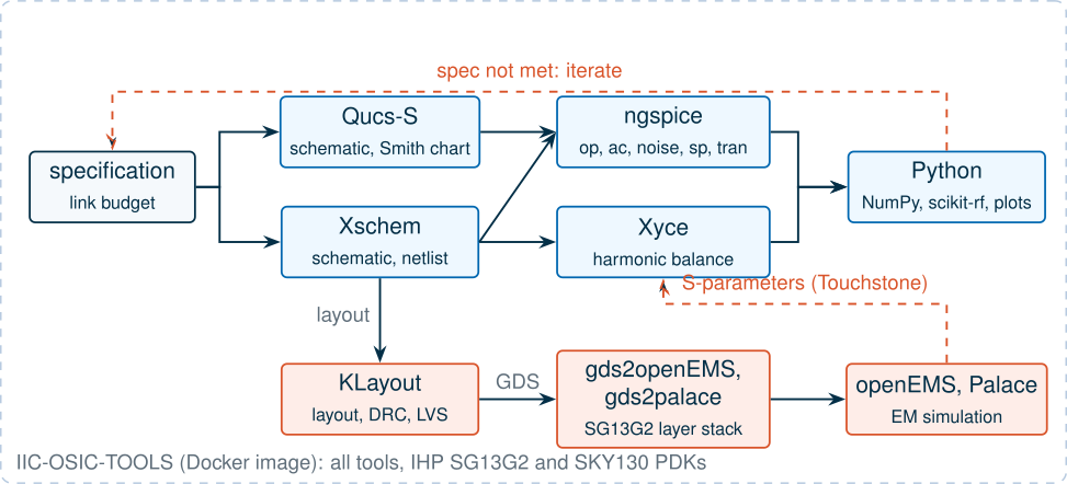
Two things make the RF flow different from the analog flow of the sibling course (The Art of Analog IC Design, Chapter 2). First, ngspice has no harmonic-balance analysis, so large-signal steady-state simulations go to Xyce, the same split the IHP Analog Academy’s 50 GHz amplifier uses [3]. Second, at RF the layout is part of the circuit: an inductor, a transmission line or the wiring around a transistor is simulated electromagnetically and enters the circuit simulation as an S-parameter file. Chapter 2 explains each analysis and when to use it.
The scripts in tools/figs/ produce every plot and number of the course. They use a small Python package, tools/rfic, that writes netlists for either PDK, runs ngspice or Xyce, and reads the results; on a laptop with Docker, it runs each simulation in the IIC-OSIC-TOOLS image automatically. The script of this chapter, for example, ran the bias sweeps and S-parameter simulations behind Figure 1.6 in a few minutes.
1.6 The course radio: a 2.4 GHz transceiver and a 50 GHz amplifier
Every chapter that designs a block designs it for one radio, so that the numbers fit together. The course radio is a 2.4 GHz transceiver in the style of Bluetooth Low Energy [184]. It uses 40 channels, 2 MHz apart, from 2402 to 2480 MHz, and Gaussian frequency-shift keying at 1 Mb/s, so its receiver needs a noise bandwidth of about 1 MHz. The receiver is a low-IF design with quadrature down-conversion; Chapter 5 chooses the IF, about 1 MHz, and derives the block specifications from a link budget. It must detect −90 dBm with a system noise figure of 8 dB or less; its LNA must reach a noise figure of 3 dB or less with at least 15 dB of gain and an input match (S11) better than −10 dB across the band, and its front end an input third-order intercept point (IIP3) of −15 dBm or more. The receiver and the synthesizer run from 1.2 V. The synthesizer locks an LC VCO at twice the LO, 4.80–4.97 GHz, to a 40 MHz crystal with a fractional-N PLL, with a phase noise of −110 dBc/Hz or less at 1 MHz offset. The transmitter delivers +10 dBm into 50 Ω at 2.44 GHz with a power-added efficiency (PAE) of at least 30 %, from a supply chosen in Chapter 16. Table 1.5 collects the specification.
Table 1.5. Specification of the course radio (typical corner, 27 °C, unless a section studies corners and temperature).
| Item | Specification | Designed in |
|---|---|---|
| Band | 2.400–2.4835 GHz ISM band; 40 channels at 2 MHz spacing, 2402–2480 MHz | Ch. 5 |
| Modulation | GFSK, 1 Mb/s; receiver noise bandwidth about 1 MHz | Ch. 5 |
| Receiver architecture | low-IF, quadrature (I/Q) down-conversion, IF about 1 MHz | Ch. 5, 10 |
| Receiver | sensitivity ≤ −90 dBm; system NF ≤ 8 dB; front-end IIP3 ≥ −15 dBm | Ch. 4, 5, 19 |
| LNA | NF ≤ 3 dB, gain ≥ 15 dB, S11 ≤ −10 dB across the band | Ch. 9 |
| Supply | 1.2 V for the receiver and synthesizer; the PA may use its own | Ch. 16 |
| Synthesizer | 40 MHz crystal; LC VCO at 2 × LO, 4.80–4.97 GHz, divided by two for I/Q; fractional-N; LO phase noise ≤ −110 dBc/Hz at 1 MHz | Ch. 11–15 |
| Transmitter | +10 dBm into 50 Ω at 2.44 GHz; PAE ≥ 30 %; harmonics suppressed by the output match | Ch. 16 |
The 50 GHz amplifier. The second project takes the course into millimetre waves. Chapter 17 designs a 50 GHz medium-power amplifier in SG13G2’s npn13G2 HBTs, following module 2 of the IHP Analog Academy [3]: bias and stability in ngspice, input matching with ideal elements, output matching and harmonic-balance simulation in Xyce, and finally layout and electromagnetic simulation in openEMS. It is the place where the two lessons of this chapter meet: at 50 GHz only the HBT has gain to spare (Figure 1.6), and every wire longer than 0.3 mm is a transmission line (Figure 1.2).
1.7 How to use this course
What you need to know. The course assumes the analog background of SkillSurf’s The Art of Analog IC Design [4]. In particular:
- MOSFET models and small-signal analysis: Chapter 4 and Chapter 5;
- gm/ID sizing and single-transistor amplifiers: Chapter 6 and Chapter 7;
- frequency response, feedback and stability: Chapter 9 and Chapter 11;
- noise: Chapter 13; and, before Part IV, phase-locked loops: Chapter 22;
- the two PDKs and the open-source toolbox: Chapter 3 and Chapter 2.
You also need phasors, two-port networks and Fourier transforms, and enough Python to run a script and change a number in it. Electromagnetics helps but is not required.
How the parts fit together. Part I gives you the language: the simulators (Chapter 2), transmission lines, S-parameters and the Smith chart (Chapter 3), noise and linearity (Chapter 4) and transceiver architectures (Chapter 5), which turns the specification of Table 1.5 into a budget for each block. Part II characterizes the components, transistors (Chapter 6), passives (Chapter 7) and matching networks (Chapter 8). Read Parts I and II in order. Parts III (the receiver), IV (the synthesizer) and V (the transmitter) can then be read in any order; each designs its blocks for the course radio. Part VI lays out and verifies the blocks and puts the radio together.
How to read a chapter. Every chapter follows the same rhythm: the physical idea, an equation, a hand calculation, a simulation with the PDK’s models, and what it means for your design. Every number comes from a script you can run and change.
Try it · The script of this chapter
tools/figs/ch01_why_rf.pydraws every figure of this chapter and simulates the three transistors:python3 tools/figs/ch01_why_rf.py gain --resim. Three experiments: (1) changeJ_MOSfrom 0.2 to 0.1 and 0.4 mA/µm: how much does Gmax at 50 GHz of the SG13G2 nMOS change, and what does it cost in current? (2) Give the HBT eight emitters (nx=8indevice_line) at the same current density: does Gmax change, as Section 1.4 claims it should not? (3) Contact the SKY130 gate fingers on one side only, \(R_g = R_\square W_f/(3\,L\,n_f)\) = 21.4 Ω: what happens to its \(f_{max}\), and to its MSG?
- Radios have moved up the spectrum for bandwidth and small antennas; the course works at 2.44 GHz (λ0 = 123 mm) and 50 GHz (λ0 = 6.0 mm).
- RF circuits are specified in power and impedance: dBm at 50 Ω interfaces. The course radio must handle signals from −90 dBm (10 µV peak) to +10 dBm (1 V peak), against a noise floor of −174 dBm/Hz.
- A wire longer than λ/10 is a transmission line: on chip that is 6.07 mm at 2.44 GHz but only 0.296 mm at 50 GHz.
- Noise, linearity, gain, frequency, power and supply voltage all trade against each other: the RF design hexagon.
- At 2.44 GHz all three transistors offer 20 dB or more of Gmax; at 50 GHz the SG13G2 nMOS has 3.6 dB and the SiGe HBT 15.8 dB, which is why the 50 GHz amplifier uses HBTs. Check a model’s parasitics before trusting it at high frequency.
- Open tools now cover the whole RF flow: Xschem, ngspice, Xyce, KLayout, openEMS, Palace and Python, all in IIC-OSIC-TOOLS.
Further reading
- B. Razavi, RF Microelectronics [6], Chapter 1: a short, lively case for why RF design is hard, and the origin of the design hexagon; T. H. Lee, The Design of CMOS Radio-Frequency Integrated Circuits [7], for the history of radio and a physical view of every block.
- D. M. Pozar, Microwave Engineering [8]: transmission lines and the microwave view of circuits; S. Voinigescu, High-Frequency Integrated Circuits [10], for SiGe and CMOS circuits up to millimetre waves.
- A. A. Abidi, “RF CMOS comes of age” [24], and J. D. Cressler, “SiGe HBT technology” [25]: how CMOS and SiGe each earned their place in radios.
- H. Pretl, Radio-Frequency Integrated Circuits [1]: an open course on the same open stack, whose scope this course follows.