Lab 3
On-Chip Inductors
Take one of Chapter 7's spirals from its layout to a model a circuit simulator can use: an electromagnetic simulation in Palace, its inductance, Q and self-resonance, a physical π model, and a rational model from vector fitting that ngspice simulates as a subcircuit.
- Run IHP’s gds2palace flow and Palace on a spiral, or start from the provided Touchstone file.
- Compute L, Q and the self-resonant frequency, single-ended and differential, from a two-port’s Y- and Z-parameters with scikit-rf.
- Fit the eight-element π model of Chapter 7 with SciPy and judge where it holds.
- Vector-fit the EM data with scikit-rf, check and enforce passivity, and verify the SPICE subcircuit in ngspice.
Contents
| Lab 3 at a glance | |
|---|---|
| Goal | L, Q and SRF of the 3-turn spiral L3 from EM data, a π-model fit and a vector-fitted ngspice model, against Chapter 7’s Tables 7.2 and 7.3 and Chapter 18’s vector fits. |
| Chapters | Chapter 7 (Sections 7.2–7.4, Eqs. 7.5–7.9, Tables 7.2 and 7.3) and Chapter 18 (Section 18.5, Eqs. 18.4–18.5) |
| Time | 2 hours, plus 10–20 minutes of computer time for the optional EM run |
| Files | tools/labs/lab3/: em_run.py (optional), inductor.py, vf_sp.cir, pi_sp.cir. Chapter 7’s layouts and results: tools/em/ch07_inductors/ (ch07_geom.py, ch07_palace.py, gds/L3.gds, L3.s2p) |
| Run time | em_run.py L3 9 min with 4 MPI processes on an 8-core laptop; inductor.py about 10 s |
Run every command in tools/labs/lab3, inside the container or from your computer with ../common/iic.sh in front of it. The course plan does steps 1–3 after Chapter 7 and steps 4–5 after Chapter 18.
Hand calculation
L3 is a symmetric octagonal spiral on TopMetal2 (Figure 7.3): \(N\) = 3 turns, \(d_{out}\) = 170 µm, \(w\) = 8 µm, \(s\) = 2.1 µm, a 1460 µm long track, TopMetal2 at 11 mΩ/□.
- Inductance. Find \(d_{in}\), \(d_{avg}\) and the fill ratio \(\rho\), then \(L\) with the modified Wheeler formula, Eq. (7.5).
- Q from the metal alone. Compute \(R_{DC} = l R_\square / w\) and the Q that \(R_{DC}\) alone would allow at 2.44 GHz, \(\omega L/R_{DC}\), with the EM inductance of 1.92 nH. The skin depth of TopMetal2 at 2.44 GHz is 1.85 µm, less than its 3 µm thickness: which way does that move Q?
- Self-resonance. Once step 3 has fitted the π model (or with Table 7.3’s L3 row), estimate the single-ended SRF. With port 2 grounded, the inductance \(L_0 + L_1\) resonates with \(C_p\) in parallel with the port-1 shunt branch; neglect \(R_{si}\), so that the branch is \(C_{ox}\) in series with \(C_{si}\).
Steps
-
The EM simulation (optional, long). The layout of L3 is
tools/em/ch07_inductors/gds/L3.gds, drawn by Chapter 7’sch07_geom.py; open it in KLayout from the container’s desktop to see the turns, the TopMetal1 crossings, the Metal1 ground frame and the two port boxes on layers 201 and 202. Then runpython3 em_run.py L3 # 4 MPI processes; EM_NP=2 python3 em_run.py L3 on a smaller machineIt uses Chapter 7’s flow (
ch07_palace.py) unchanged: IHP’s gds2palace [206] merges the polygons, models each metal as an impedance sheet of its thickness and conductivity in IHP’sSG13G2_200um.xmlstack-up, meshes the volume with gmsh (5 µm on the conductors) and writes the configuration for Palace [197], which solves with second-order elements and an adaptive frequency sweep from 0.01 to 30 GHz. The mesh goes totools/_work/lab3_em/L3/and the result toout/L3_em.s2p; Chapter 7’s file is not touched. Palace peaked at 4.1 GB of memory with four processes: give Docker at least 6 GB, or use two processes. If you skip this step, the next steps use Chapter 7’sL3.s2p, which this flow produced. -
L, Q and SRF. Run
python3 inductor.py(python3 inductor.py L2for another spiral of the family). It reads the Touchstone file into a scikit-rfNetworkand applies Eq. (7.8) twice:z_se = 1 / ind.y[:, 0, 0] # single-ended: port 2 grounded z = ind.z z_d = z[:, 0, 0] + z[:, 1, 1] - z[:, 0, 1] - z[:, 1, 0] # differential: ground floating L, Q = z_se.imag / w, z_se.imag / z_se.real # and the SRF where Im(z) crosses zero -
The π model. The script fits the eight elements of Figure 7.4b, \(L_0\), \(L_1\), \(R_{dc}\), \(R_1\), \(C_p\), \(C_{ox}\), \(R_{si}\) and \(C_{si}\), with
scipy.optimize.least_squares[178]: the series branch to \(-1/Y_{12}\) and the shunt branch to \(Y_{11} + Y_{12}\), with relative errors on real and imaginary parts, from the lowest frequency to 0.8 times the SRF, from three starting points, as Chapter 7 did [98]. -
Vector fitting. Next it fits a rational model to the S-matrix with scikit-rf [215], Eq. (18.4) [172]:
from skrf.vectorFitting import VectorFitting
vf = VectorFitting(ind)
vf.auto_fit()                    # chooses the number of real and complex poles
vf.get_rms_error(), vf.is_passive()
vf.passivity_enforce(n_samples=2000)
vf.write_spice_subcircuit_s("out/L3_vf.sp", fitted_model_name="l3_vf")
A rational model can be slightly active: if the largest singular value of its S-matrix exceeds one at any frequency, a transient simulation can oscillate. The fit of L3 exceeds one by 1 × 10⁻⁵ between 12 and 54 MHz.
passivity_enforceperturbs the residues until it does not; with its default of 200 frequency samples it reports that it failed and suggests more, hencen_samples=2000. -
Both models in ngspice. The script writes
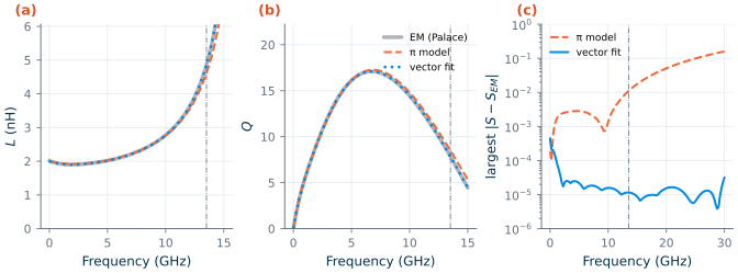
out/model.incwith two subcircuits,ind_vf(the vector fit) andind_pi(the π model), and runsvf_sp.cirandpi_sp.cir, anspanalysis of each between two 50 Ω ports. It reads the results back, interpolates them onto the EM frequencies and prints the largest difference from the EM S-parameters, and L, Q and SRF of each (Figure L3.1). Openout/L3_vf.sp: the subcircuit holds only resistors, capacitors and controlled sources, the realization of Eq. (18.5).
Checkpoint
Table L3.1. Lab 3 results for L3 (tolerance ±1 in the last digit; hand values: L within 12 %, SRF within 2 %; your own EM run against the provided file: ±1 in the last digit of every row).
| Quantity | Lab 3 | Chapter |
|---|---|---|
| Hand: \(d_{in}\), \(d_{avg}\), \(\rho\); Wheeler \(L\) | 113.6 µm, 141.8 µm, 0.199; 2.12 nH | 2.12 nH (Table 7.2) |
| Hand: \(R_{DC}\); \(\omega L/R_{DC}\) at 2.44 GHz | 2.01 Ω; 14.6 | 2.01 Ω (Table 7.2) |
| EM run: unknowns (second order), adaptive samples, solve time, peak memory | 329 364, 7, 530 s (4 processes), 4.1 GB | 329 364, 7 (Chapter 7 run) |
EM run against Chapter 7’s L3.s2p: largest \(\vert\Delta S\vert\) |
6 × 10⁻¹⁰ | |
| \(L\) at 1 GHz; \(R\) at 0.01 GHz | 1.92 nH; 1.74 Ω | 1.92 nH; 1.74 Ω (Table 7.2) |
| Q at 2.44 GHz; at 4.88 GHz (differential) | 10.6; 16.0 (17.7) | 10.6; 16 (17.7) |
| Peak Q, at | 17.1, 6.75 GHz | 17.1, 6.75 GHz |
| SRF (differential) | 16.9 (18.7) GHz | 16.9 (18.7) GHz |
| π model: \(L_0\), \(L_1\), \(R_{dc}\), \(R_1\) | 1850 pH, 130 pH, 1.75 Ω, 1.03 Ω | the same (Table 7.3) |
| π model: \(C_p\), \(C_{ox}\), \(R_{si}\), \(C_{si}\); fit to | 26.2 fF, 40.4 fF, 1540 Ω, 34.9 fF; 13.5 GHz | the same (Table 7.3) |
| Hand: SRF from the π values | 16.9 GHz | |
| Vector fit: poles; rms error as fitted / after passivity enforcement | 5 real + 2 complex pairs; 2.2 × 10⁻⁵ / 1.3 × 10⁻⁴ | Ch. 18 (three-ports, own code): 2 real + 5 or 7 pairs; 1.97 / 1.09 × 10⁻⁴ |
| Vector fit: largest singular value as fitted / passive (DC to 300 GHz) | 1.00001 / 0.99948 | Ch. 18: ≤ 1.002, then scaled |
| ngspice, vector fit: largest \(\vert\Delta S\vert\) to 30 GHz; L and Q at 2.44 GHz; SRF | 4.5 × 10⁻⁴; 1.90 nH, 10.6; 16.9 GHz | Ch. 18: within 6 × 10⁻⁴ |
| ngspice, π model: largest \(\vert\Delta S\vert\) to 13.5 / 30 GHz; L and Q at 2.44 GHz; SRF | 0.011 / 0.16; 1.92 nH, 10.5; 17.4 GHz | Q 10.5, SRF 17.4 GHz (Ch. 7) |
The lab reproduces every number of Chapter 7 for L3, and the EM run reproduces Chapter 7’s Touchstone file to the tenth decimal: the flow is deterministic for a given mesh and solver. Chapter 18 used its own implementation of vector fitting on three-port networks to 160 GHz, so its numbers are a yardstick, not a target: scikit-rf’s fit of this two-port is as accurate in ngspice (4.5 × 10⁻⁴ against 6 × 10⁻⁴) and is made passive by perturbing the residues rather than by scaling. Your hand calculations should give \(d_{in}\) = 113.6 µm, \(\rho\) = 0.199, \(L\) = 2.12 nH (10 % above the EM value, as Chapter 7 found), \(R_{DC}\) = 2.01 Ω, a metal-only Q of 14.6 against 10.6, and, with \(C_{ox}\) in series with \(C_{si}\) (18.7 fF) plus \(C_p\), 45.0 fF and an SRF of 16.9 GHz.
Questions
- The EM resistance at 0.01 GHz, 1.74 Ω, is 13 % below \(lR_\square/w\). Chapter 7 attributes the difference to how gds2palace represents a metal. What is it, and why does it not matter at 2.44 GHz?
- Q at 2.44 GHz is 10.6, not the 14.6 of the metal alone. Using Eq. (7.9) and the π values, how much of the difference is the skin and proximity effect in the series branch, and how much the substrate?
- The differential Q at 4.88 GHz is 17.7 against 16.0 single-ended, and the differential SRF 1.8 GHz higher. Explain both with the shunt branches of the π model.
- The π model is fitted to 13.5 GHz and is 0.16 off in S at 30 GHz, while the vector fit has no such limit. What does the π model offer that a vector fit does not? When would you use each?
- The vector fit needed only two complex pole pairs and five real poles for 0.01–30 GHz. What physical behaviour do the real poles describe, and why does the fit slightly exceed passivity just near DC?
Extension
- Another spiral. Run
python3 inductor.py L4(or the EM runpython3 em_run.py L4first, about 20 minutes) and compare with the L4 column of Table 7.2: SRF 8.12 GHz, peak Q 12.4 at 3.5 GHz. How many poles doesauto_fitchoose now, and why? - Fixed model order. Replace
vf.auto_fit()byvf.vector_fit(n_poles_real=1, n_poles_cmplx=1), then byvf.vector_fit(n_poles_real=2, n_poles_cmplx=3). Plotvf.get_rms_error()against the number of poles, and watch the ngspice error of panel (c). How few poles still give \(\vert\Delta S\vert\) < 10−3? - A transient with the EM model. Put the subcircuit
ind_vfofout/model.incin parallel with a 1 pF capacitor, charge the capacitor to 0.1 V and let the tank ring (tran 1p 5n uic). Measure the frequency and the decay of the envelope, and compare \(Q\) from the decay with the inductor’s Q at that frequency. Repeat withind_pi.