Chapter 16
Power Amplifiers
The power amplifier is the one block of a radio whose job is to waste as little power as possible while handling the most. This chapter builds the PA from the conduction angle up: the efficiency classes, the load line and why it is not a conjugate match, switching amplifiers, linearity and back-off, breakdown and stacking, and the techniques that recover efficiency. It ends with the course PA at 2.44 GHz in SG13G2, where the on-chip inductors decide whether the efficiency target is met.
- Define output power, collector efficiency and PAE, and the linearity and spurious-emission metrics a PA must meet.
- Derive the efficiency and output power of classes A, AB, B and C from the conduction angle, and the optimum load from the load line.
- Design a class-E stage with Sokal’s equations and explain zero-voltage switching.
- Explain how breakdown limits a PA’s supply, and how cascodes, stacking and power combining work around it.
- Design and simulate a 2.44 GHz SiGe cascode PA with an output network made of SG13G2 spirals, and judge it against the course specification.
Contents
- 16.1 What a power amplifier must do
- 16.2 Classes A, B, AB and C
- 16.3 Load lines and load-pull
- 16.4 Switching amplifiers: classes D, E and F
- 16.5 Linearity: AM-AM, AM-PM and back-off
- 16.6 Breakdown, stacking and power combining
- 16.7 Efficiency enhancement and linearization
- 16.8 The course PA at 2.44 GHz
- Further reading
16.1 What a power amplifier must do
A PA takes a modulated carrier of a few milliwatts or less from the upconverter or the synthesizer and delivers the transmit power to the antenna. Three groups of numbers describe it: how much power, at what cost, and how cleanly.
Power and efficiency. The output power \(P_{out}\) is the power at the carrier frequency delivered to the load, usually 50 Ω. The supply delivers \(P_{DC}\); whatever does not reach the load heats the transistor and the matching network. Two efficiencies are in use:
\[\eta = \frac{P_{out}}{P_{DC}}, \tag{16.1}\] \[\mathrm{PAE} = \frac{P_{out} - P_{in}}{P_{DC}} = \eta\left(1 - \frac{1}{G}\right). \tag{16.2}\]The collector (drain) efficiency \(\eta\) ignores the input power; the power-added efficiency (PAE) charges it to the PA. With a power gain \(G\) of 20 dB the two differ by 1 %; with 6 dB of gain, by a quarter. PAE is the honest number for a PA whose driver is part of the same chip.
Linearity. The 1 dB compression point (P1dB, Chapter 4) is where the gain has dropped by 1 dB. A PA is also described by two curves against the input amplitude: the gain (AM-AM conversion) and the insertion phase (AM-PM conversion). For a signal with a varying envelope they produce spectral regrowth, measured as the adjacent-channel power ratio (ACPR or ACLR, the power leaked into the next channel in dBc), and in-band distortion, measured as the error-vector magnitude (EVM, Chapter 5). The standard sets both, and a spectral mask on the whole output spectrum.
Harmonics. A transistor driven hard enough to be efficient produces strong harmonics, and the output network must remove them. Regulations limit spurious emissions; for 2.4 GHz equipment in Europe the limit from 1 to 12.75 GHz is −30 dBm in 1 MHz [189], so at +10 dBm the harmonics must be at least 40 dB below the carrier. The course radio adds its own reason (Chapter 5): the second harmonic at 4.88 GHz lies on the VCO.
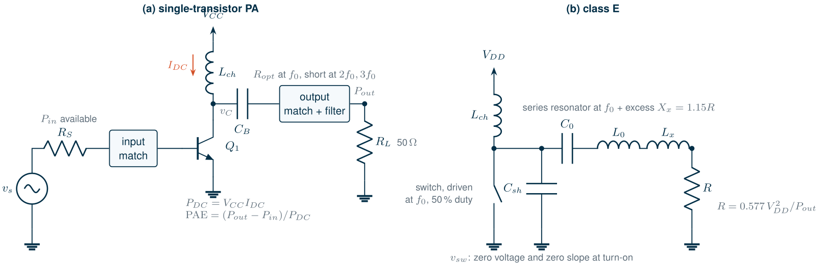
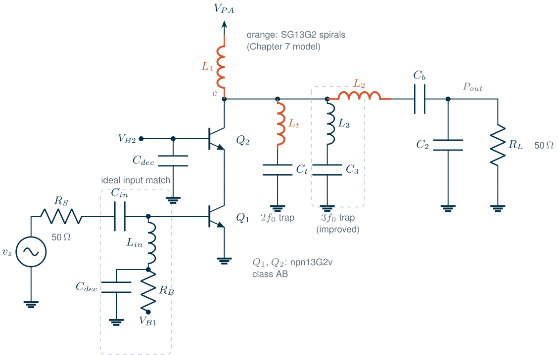
Figure 16.1a shows the generic stage. The choke feeds the collector from the supply, the DC block keeps the supply off the load, and the output network does two jobs at once: it transforms the 50 Ω load into the resistance the transistor needs at the carrier \(f_0\), and it presents a low impedance at \(2f_0\) and \(3f_0\).
Table 16.1. The course transmitter's PA specification (from the course radio of the Preface and Chapter 5).
| Item | Target | Origin |
|---|---|---|
| Output power | +10 dBm into 50 Ω at 2.44 GHz (2.402–2.480 GHz) | course radio |
| PAE at +10 dBm | ≥ 30 % | course radio |
| 2nd and 3rd harmonic | ≤ −40 dBc (−30 dBm at +10 dBm) | spurious limit [189]; 2f0 on the VCO |
| Linearity | none beyond the mask: GFSK has a constant envelope | Chapter 5 |
| Supply | separate PA supply allowed | course radio |
Because BLE’s GFSK has a constant envelope (Chapter 5), the course PA may run in compression; its AM-PM matters only through the phase noise and pulling it might add. A Wi-Fi PA would have to meet an EVM and back off by the 9.6 dB PAPR of OFDM, which is the subject of Section 16.5.
16.2 Classes A, B, AB and C
The first PA classes differ only in the bias, which sets how much of each period the transistor conducts: the conduction angle \(\alpha\). Assume the output network passes only the fundamental, so the collector voltage is a sinusoid of amplitude \(V_1\) around \(V_{CC}\), and the collector current is a sinusoid clipped at zero, a pulse of peak \(I_{max}\) that lasts \(\alpha\) of the 360° period (Figure 16.2a). Its Fourier series gives the DC current, which sets \(P_{DC}\), and the fundamental, which sets \(P_{out}\) [13, 6]:
\[I_{DC} = \frac{I_{max}}{2\pi}\,\frac{2\sin(\alpha/2) - \alpha\cos(\alpha/2)}{1 - \cos(\alpha/2)}, \qquad I_1 = \frac{I_{max}}{2\pi}\,\frac{\alpha - \sin\alpha}{1 - \cos(\alpha/2)}. \tag{16.3}\]With \(P_{out} = V_1 I_1/2\) and \(P_{DC} = V_{CC} I_{DC}\), the efficiency is
\[\eta = \frac{V_1}{V_{CC}}\,\frac{\alpha - \sin\alpha}{2\left[2\sin(\alpha/2) - \alpha\cos(\alpha/2)\right]}. \tag{16.4}\]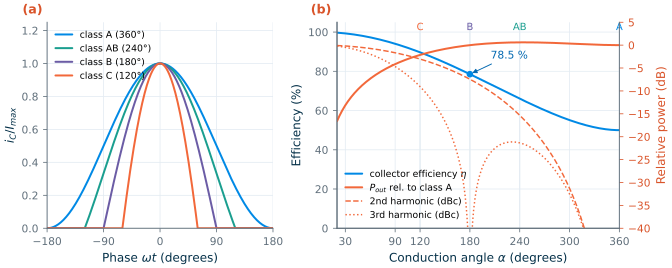
Figure 16.2b evaluates Eqs. (16.3)–(16.4) at full swing, \(V_1 = V_{CC}\):
- Class A (\(\alpha\) = 360°): the transistor always conducts, the current has no harmonics, and the efficiency is at most 50.0 %. It is the linear reference.
- Class B (180°): biased at the threshold, the transistor conducts for half the period. The efficiency rises to \(\pi/4\) = 78.5 % at the same output power as class A, but the half-sine current has a second harmonic only 7.4 dB below the fundamental.
- Class AB (between): a small quiescent current. At 240° the efficiency is 66.1 % and the output power 0.61 dB above class A, close to its maximum of 0.61 dB at 245°; the second harmonic of the current is −15.3 dBc. Almost every linear PA is class AB.
- Class C (below 180°): at 120° the efficiency is 89.7 % but the output power has fallen by 2.14 dB for the same peak current, and the harmonics are large. Efficiency approaches 100 % only as the output power approaches zero.
The analysis treats the transistor as an ideal transconductor that never saturates. A real collector cannot swing below its knee voltage \(V_{knee}\), so \(V_1 \le V_{CC} - V_{knee}\) and every efficiency falls by the factor \(V_1/V_{CC}\); at the low supplies of a SiGe or CMOS PA that factor is the first thing to lose.
16.3 Load lines and load-pull
The class fixes the shape of the current; the load fixes how much power comes out. For maximum power the collector voltage should swing from \(V_{knee}\) to \(2V_{CC} - V_{knee}\) just as the fundamental current reaches its largest value. The load that does both is the optimum load, set by the load line [13]:
\[R_{opt} = \frac{(V_{CC} - V_{knee})^2}{2P_{out}}. \tag{16.5}\]Key equation · The load-line match
\(R_{opt} = \frac{(V_{CC} - V_{knee})^2}{2P_{out}}\) (16.5): the supply and the power fix the load, not the transistor’s output impedance.
This is not a conjugate match. A conjugate match maximizes the power transferred from a linear source with a fixed internal resistance; a PA’s limits are its current and voltage swings, and its output resistance is far higher than \(R_{opt}\). For the course PA’s cascode the small-signal output impedance at 2.44 GHz is 44.3 − j934 Ω: conjugately matched, the collector would see hundreds of ohms, the voltage would clip long before the current reached its limit, and the output power would be a fraction of what Eq. (16.5) allows. The reactive part of the output impedance is still tuned out, so that the intrinsic collector sees a resistance.
Worked example 16.1 · The load for +10 dBm
The course PA (Section 16.8) is a cascode of two
npn13G2vHBTs on a 2.0 V supply. The cascode’s knee is the saturation voltage of both transistors, about 0.6 V at the currents involved (Section 16.8 reads it from the simulated waveform). If the network loses about 1 dB, the collector must deliver +11 dBm, 12.6 mW, and Eq. (16.5) gives \(R_{opt}\) = (2.0 − 0.6)²/(2 × 12.6 mW) = 78 Ω. The load is close to 50 Ω, so the output network needs little impedance transformation, which keeps its loss low.
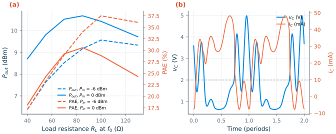
Load-pull finds the optimum load by measurement or simulation: the load impedance at \(f_0\) is varied over the Smith chart (with the harmonics terminated in a fixed way), and the output power and PAE are drawn as contours. The power and PAE optima are near each other but not at the same point, and both move with the drive level. Figure 16.7a shows a one-dimensional version for the course PA: an ideal tuner that shorts the harmonics and presents a resistance \(R_L\) at \(f_0\), swept from 40 to 130 Ω at two drive levels. Figure 16.8a draws the contours over a small grid of complex loads.
16.4 Switching amplifiers: classes D, E and F
Eq. (16.4) has a ceiling because the transistor carries current while voltage is across it. A switching amplifier removes the overlap: the transistor is driven as a switch, either fully on (current, no voltage) or fully off (voltage, no current), and the output network turns the switched waveform into a sinusoid in the load [165].
Class D switches the output node between the supply and ground with two transistors (an inverter), and a series-resonant filter passes the fundamental of the square wave to the load. Ideally 100 % efficient, it loses \(CV_{DD}^2 f_0\) every period to the capacitance \(C\) of the switching node, which is why class D, and its digital descendants, are used mainly below a few gigahertz in fine-line CMOS.
Class E uses one transistor and absorbs its capacitance into the network (Figure 16.1b). A shunt capacitor \(C_{sh}\) (including the transistor’s) and a series resonator with an excess reactance \(X_x\) shape the switch voltage so that, just before the switch closes, the voltage has returned to zero with zero slope: zero-voltage switching (ZVS) with zero \(dv/dt\). The capacitor is never discharged through the switch, and small errors in the timing cost little. For a 50 % duty cycle and a high loaded Q, Sokal and Sokal’s design equations are [162, 163]
\[R = \frac{8}{\pi^2 + 4}\,\frac{V_{DD}^2}{P_{out}} = 0.577\,\frac{V_{DD}^2}{P_{out}}, \quad C_{sh} = \frac{0.184}{\omega R}, \quad X_x = 1.15\,R, \quad v_{sw,max} = 3.56\,V_{DD}. \tag{16.6}\]Worked example 16.2 · A class-E stage for +10 dBm into 50 Ω
For \(R\) = 50 Ω and 10 mW, Eq. (16.6) gives \(V_{DD}\) = 0.931 V, \(C_{sh}\) = 0.24 pF and \(L_x\) = \(X_x/\omega\) = 3.76 nH; a series resonator with a loaded Q of 5 adds \(L_0\) = 16.3 nH and \(C_0\) = 0.261 pF. Eq. (16.6) assumes a high loaded Q and an infinite choke; for \(Q_L\) = 5 and a 50 nH choke, solving the circuit exactly for zero voltage and zero slope at turn-on moves \(C_{sh}\) to 0.314 pF and \(L_x\) to 3.68 nH. The switch must stand 3.56 × 0.931 = 3.3 V.
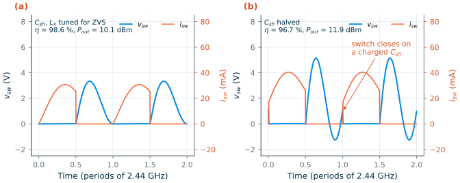
Figure 16.3a shows the tuned stage in an ngspice transient. The switch voltage peaks at 3.34 V, 3.59 \(V_{DD}\), and lands on zero with zero slope; the current peaks at 30.8 mA, 2.77 times the DC current of 11.1 mA, and the stage delivers 10.08 dBm with 98.6 % efficiency, the rest lost in the 0.5 Ω switch. With \(C_{sh}\) halved (Figure 16.3b) the switch closes on 0.95 V, the peak voltage rises to 5.14 V, and the energy \(\tfrac12 C_{sh} v^2\) dumped every period costs 0.173 mW: the efficiency falls to 96.7 %. The ideal switch flatters class E. A real transistor has a finite on-resistance, a capacitance that is nonlinear, and needs a large, fast drive, whose power counts in the PAE; and its peak voltage is 3.56 \(V_{DD}\), more than any single SG13G2 device stands at a useful supply (Section 16.6).
Class F shapes the waveforms with harmonic resonators instead of a switch. The output network presents an open circuit at the odd harmonics and a short at the even ones, so the collector voltage approaches a square wave while the current is a half sine, and they do not overlap [164]. With only the third harmonic controlled, the maximally flat voltage has \(V_1 = \tfrac98 V_{CC}\) and the efficiency of class B rises from 78.5 % to \(\tfrac98 \times 78.5\,\%\) = 88.4 %. Each controlled harmonic costs a resonator, and on chip each resonator costs loss.
16.5 Linearity: AM-AM, AM-PM and back-off
A PA is linear only well below compression. Its two characteristic curves, gain and phase against input power, describe a memoryless amplifier: the AM-AM curve compresses as the collector swing reaches the knee and the supply, and the AM-PM curve moves because the transistor’s capacitances and the base-emitter impedance change with the drive. For a constant-envelope signal both are harmless: every sample sees the same gain and phase. For a signal whose envelope varies, every sample sees a different gain and phase, and the result is EVM and spectral regrowth.
The remedy without extra circuits is back-off: run the PA with its average output a PAPR below its saturated power so that the peaks are not clipped. Back-off is expensive. With the swing scaled down, Eq. (16.4) gives
\[\eta_A = 0.5\,\frac{P_{out}}{P_{max}}, \qquad \eta_B = \frac{\pi}{4}\sqrt{\frac{P_{out}}{P_{max}}}. \tag{16.7}\]At the 9.6 dB back-off of OFDM (Chapter 5), an ideal class-B PA drops from 78.5 % to 26.0 % and class A from 50 % to 5.5 %. The course radio’s GFSK avoids the problem entirely: it can run the PA at its most efficient drive. Section 16.7 describes how transmitters for envelope-varying signals recover the efficiency.
16.6 Breakdown, stacking and power combining
For a given output power, Eq. (16.5) trades supply against load. A high supply and a high \(R_{opt}\) would be ideal, because then the network barely transforms the load and the currents, and the losses in every series resistance, are small. Breakdown stops this. A class-A or class-B collector swings to about \(2V_{CC}\), so \(V_{CC}\) must stay below half the breakdown voltage (Chapter 6). For the SG13G2 devices:
npn13G2: \(BV_{CEO}\) = 1.6 V, \(BV_{CBO}\) = 4.8 V; thenpn13G2vtrades speed for voltage, \(BV_{CEO}\) = 2.5 V and \(BV_{CBO}\) = 8.5 V (2.2 V and 7 V minimum) [200].- 1.2 V MOSFETs: \(BV_{DSS}\) = 2.7 V typical, 2.0 V minimum; the 3.3 V devices reach 6.1 V but have only 16.0 GHz of \(f_T\).
\(BV_{CEO}\) is a worst case: it assumes an open base, where the holes from avalanche multiplication in the collector are multiplied again by \(\beta\). A base driven from a low impedance carries those holes away, and the usable collector voltage rises towards \(BV_{CBO}\) (Chapter 6). This is the key to the cascode PA: the common-base transistor’s base is held at a fixed voltage by a large capacitor, so its collector can swing beyond \(BV_{CEO}\), while the common-emitter transistor below it sees only a small swing. Stacking extends the idea to three or more transistors in series, each gate or base driven by a capacitive divider so that the output swing divides evenly among them [168]; it is how fine-line CMOS PAs reach watts.
Common pitfall · Forgetting where the avalanche current goes
Above \(BV_{CEO}\) the base current of an HBT reverses (Chapter 6, at 2.60 V for
npn13G2v). A cascode base biased through a resistor, or from a bias circuit that can only source current, lets the base voltage float up and the transistor run away. The bias network of a common-base PA transistor must sink current at DC and have a low impedance at RF.
When one stage cannot deliver the power within its limits, several are combined. Transformers on chip add the voltages of several push-pull stages in series, which also transforms the load: Aoki et al.’s distributed active transformer combined four push-pull pairs into one secondary loop on a CMOS chip [108]. Chapter 7’s stacked transformer, with \(k\) ≈ 0.72, is the building block, and its loss counts like that of any matching network. At the course PA’s 10 mW none of this is needed; at the watt level of a cellular PA, or for the 50 GHz amplifier of Chapter 17, it is.
16.7 Efficiency enhancement and linearization
Four architectures keep the efficiency high in back-off; one digital technique keeps a PA linear near compression. All are surveyed by Raab et al. [165], and Figure 16.4 sketches each.
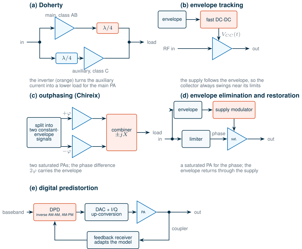
- Doherty amplifier [166]. A main amplifier (class AB) and an auxiliary amplifier (class C) are combined through a quarter-wave inverter. At low power only the main amplifier runs, into a doubled load, so it saturates, and is efficient, 6 dB below the peak power. Above that point the auxiliary amplifier turns on and its current lowers the main amplifier’s load (load modulation). The efficiency stays near its peak over the top 6 dB, at the price of bandwidth (the inverter is a quarter wave long) and a more complex layout.
- Envelope tracking [169]. A fast DC-DC converter makes the supply follow the envelope, so the collector always swings close to its limits. The converter’s own efficiency and bandwidth (several times the signal bandwidth) set the result.
- Outphasing [167]. The signal is split into two constant-envelope signals whose phase difference carries the envelope; two saturated, efficient PAs amplify them and a combiner adds them. Chireix’s compensating reactances recover the efficiency of the combiner in back-off.
- Envelope elimination and restoration (polar transmission) [72]. A saturated PA amplifies the phase-modulated carrier and the envelope modulates its supply. Chapter 5’s polar transmitter is the modern form.
- Digital predistortion (DPD) [170]. A digital model of the PA’s AM-AM and AM-PM, often with memory, distorts the baseband signal with the inverse, so that the cascade is linear. It lets a PA run with less back-off, which is where the efficiency comes from; it needs a feedback receiver to adapt the model.
What this means for your design
The course radio needs none of these: its GFSK runs the PA at its most efficient drive. They become necessary the moment the same transmitter must carry an OFDM signal, where a PA with 40 % peak efficiency averages a quarter of that in back-off.
16.8 The course PA at 2.44 GHz
Device, supply and bias
The target is modest, +10 dBm, so one transistor pair is enough; the questions are breakdown and loss. A single npn13G2 would need \(V_{CC}\) ≈ 0.8 V to keep its collector below \(BV_{CEO}\), and \(R_{opt}\) ≈ 20 Ω after the knee, a lossy transformation from 50 Ω. A cascode of two npn13G2v on a separate 2.0 V supply lets the load line sit near 50 Ω (Worked example 16.1). The common-base transistor’s base is held at 1.4 V by an ideal source (in silicon: a bias circuit that can sink current, decoupled by a large MIM capacitor), so its collector-base voltage stays far below \(BV_{CBO}\); its collector-emitter voltage exceeds \(BV_{CEO}\) at the peak, which is exactly the case where the low base impedance is required (Section 16.6). The npn13G2v is slow, \(f_T\) = 104 GHz, but forty times faster than the carrier, and Chapter 6 showed that it holds 2.5 V where the npn13G2 holds 1.6 V.
Each transistor is four npn13G2v instances of \(N_x\) = 4 fingers (\(l_E\) = 2.5 µm) in parallel, 4.8 µm² of emitter, so that the peak current stays near the current density where the device is fast. The model is scaled around \(N_x\) = 4, and a single instance with \(N_x\) = 16 made both ngspice and Xyce fail in transient analysis, so the parallel instances are also the robust choice. The common-emitter base is biased at 0.80 V, a quiescent current of 5.67 mA: class AB. A 50 Ω resistor from the base to the bias source terminates the input. It costs gain but makes the stage stable for any passive source and load from 0.16 to 28 GHz, where the μ-factor of Chapter 3 is above 1. Below 0.16 GHz μ dips to 0.99999: so close to 1 that only a lossless termination could make the stage oscillate, but a reason not to let the bias and supply networks look like pure reactances there. Without a matching network the stage gives \(S_{11}\) = −13.0 dB at 2.44 GHz and a small-signal gain into 50 Ω of 18.4 dB. (Figure 16.5.)
The load
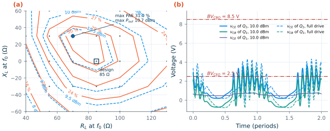
An ideal tuner finds the load: a lossless resonator at the collector shorts every harmonic and feeds the supply, and a series R + jX sets the load at \(f_0\). Figure 16.7a shows the output power and PAE against \(R_L\) at two input powers. At −6 dBm the PAE peaks at 37.5 % with 100 Ω (9.56 dBm out); at 0 dBm it peaks at 30.6 % with 85 Ω, where the stage delivers 10.68 dBm. Below 70 Ω the drive cannot supply the current the load line asks for, and the power falls (8.70 dBm at 40 Ω); above 100 Ω the voltage clips first. The design uses \(R_{opt}\) = 85 Ω, close to the 78 Ω of Worked example 16.1. A coarse two-dimensional load-pull at 0 dBm of input (Figure 16.8a: six resistances from 40 to 130 Ω, reactances from −60 to +60 Ω in steps of 30 Ω) puts the optimum of both power and PAE at the grid point 70 + j30 Ω, 10.73 dBm and 31.0 %. At 85 Ω the stage gives 10.68 dBm and 30.6 %. The contours are flat near the top, so the resistive load costs 0.4 points of PAE, less than the grid resolves; in compression the power and PAE optima coincide on this grid. Note the ceiling: even with every harmonic shorted and no network loss, this stage reaches less than 40 % PAE, because the cascode’s knee takes 0.6 V of the 2.0 V supply and the class-AB current carries a quiescent part. Chapter 8’s example match assumed an npn13G2 on 0.8 V with \(R_{opt}\) = 10.6 Ω; the 2.0 V cascode raises the load to 85 Ω, so this network transforms much less.
The output network
The network of Figure 16.5 has three spirals. \(L_1\) feeds the supply and resonates the collector capacitance; on chip it cannot be a choke, because the largest spiral of Chapter 7’s family, 4.94 nH, has only 76 Ω of reactance at 2.44 GHz. The trap \(L_t\)–\(C_t\) is series-resonant at 4.88 GHz, a short for the second harmonic, and capacitive at 2.44 GHz, where it is the tank capacitor of \(L_1\) (a harmonic trap that is also part of the match). \(L_2\) with \(C_2\) is a low-pass L-section that sets the real part of the load and attenuates the harmonics again; \(C_b\) (10 pF) blocks the DC.
Every spiral loses power. A shunt inductor of reactance \(X_L\) across \(R_{opt}\) dissipates the fraction \(R_{opt}/(Q_L X_L)\) of the power, and an L-section of network Q \(Q_n\) about \(Q_n/Q_L\) [7]:
\[\eta_{net} \approx 1 - \frac{Q_n}{Q_L}, \qquad \eta_{feed} \approx 1 - \frac{R_{opt}}{Q_L X_L}. \tag{16.8}\]With the Chapter 7 spirals (\(Q\) = 8–12 at 2.44 GHz) each term costs several per cent; with off-chip inductors (\(Q\) ≈ 40) a quarter as much. The element values come from design_net() in the script: for each pair of \(L_1\) and \(L_t\) on a grid, \(C_t\) tunes the trap to 4.88 GHz and \(L_2\), \(C_2\) are solved so that the collector sees the chosen load at 2.44 GHz; among the solutions that attenuate the second harmonic by at least 36 dB relative to the fundamental (for equal collector currents), the one with the lowest loss wins. The matching theory behind the L-section is in Chapter 8. Table 16.2 lists the three versions: the Chapter 7 spirals (tools/figs/_ch07_inductor.py, π models with skin effect and substrate), ideal inductors with Q = 40 standing for off-chip SMD parts, and lossless inductors. Its last three rows add harmonic traps to the off-chip version (“A third-harmonic trap”, below).
Table 16.2. The output network for a collector load of 85 Ω at 2.44 GHz (device output capacitance 69.7 fF absorbed): element values, network efficiency at 2.44 GHz and 2f0 and 3f0 rejection (output voltage at 4.88 or 7.32 GHz relative to 2.44 GHz for equal collector currents), from `design_net()` and, for the last three rows, `design_net_h3()`.
| Version | L1 | Lt, Ct | L2 | C2 | Cb | 3f0 trap L3, C3 | Network efficiency | 2f0 rejection | 3f0 rejection |
|---|---|---|---|---|---|---|---|---|---|
| On-chip spirals (Ch. 7 model) | 4.3 nH | 0.996 nH, 1.08 pF | 4.57 nH | 0.227 pF | 10 pF | – | 70.7 % (−1.50 dB) | −38.9 dB | −24.0 dB |
| Off-chip inductors, Q = 40 | 3.7 nH | 0.817 nH, 1.30 pF | 4.01 nH | 0.276 pF | 10 pF | – | 91.4 % (−0.39 dB) | −53.6 dB | −22.7 dB |
| Lossless inductors | 4.3 nH | 0.45 nH, 2.36 pF | 3.38 nH | 2.79 pF | 10 pF | – | 100 % | ideal short | −41.4 dB |
| Off-chip, 3f0 trap at the output (replaces C2) | 3.7 nH | 0.817 nH, 1.30 pF | 4.00 nH | – | 10 pF | 1.94 nH, 0.244 pF | 91.4 % (−0.39 dB) | −53.9 dB | −58.8 dB |
| Off-chip, 3f0 trap at the collector | 4.6 nH | 3.28 nH, 0.324 pF | 3.76 nH | 0.194 pF | 10 pF | 0.50 nH, 0.945 pF | 93.3 % (−0.30 dB) | −41.2 dB | −61.1 dB |
| Off-chip, 3f0 trap at the collector, 2f0 trap L4, C4 at the output (replaces C2) | 4.6 nH | 3.28 nH, 0.324 pF | 3.74 nH | 7.52 nH, 0.141 pF (L4, C4) | 10 pF | 0.50 nH, 0.945 pF | 93.2 % (−0.30 dB) | −66.3 dB | −62.2 dB |
The spirals lose almost 30 % of the power before it reaches the antenna, three times as much as Q = 40 inductors. The loss is spread over all three spirals: the feed inductor across the 85 Ω load (Eq. 16.8, with \(X_L\) ≈ 66 Ω and Q ≈ 11.6, about 11 %), the series inductor that carries the full output current, and the trap. Capacitors are ideal in all three versions; Chapter 7’s MIM capacitors have Q of 87 or more at 4.88 GHz with a good feed, so they would add a few tenths of a decibel.
Simulated performance
Which simulator. Xyce harmonic balance converged on this circuit only from the DC solution, and only up to −14 dBm of input (3.53 dBm out), with numfreq = 9; its transient-assisted start, and the HB of a single 16-finger npn13G2v instance, did not converge at all. The large-signal results are therefore ngspice transients of 60 periods at 2.44 GHz, with the harmonics taken from an FFT of the last 10 periods. Where both run, the two agree within 0.01 dB: 2.22 and 2.23 dBm at −16 dBm of input, 3.53 and 3.53 dBm at −14 dBm (HB values first). Self-heating of the HBTs is on in both.
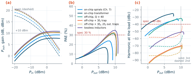
Figure 16.6 shows the three versions, and in orange the improved network of the next subsection. With the on-chip network the small-signal gain is 19.16 dB, the output-referred P1dB 2.4 dBm (input −15.8 dBm), and the output saturates at 9.2 dBm: the PA never reaches +10 dBm, and its PAE peaks at 23.8 % at 8.3 dBm. With Q = 40 inductors the PA delivers +10 dBm at −1.5 dBm of input, a gain of 11.5 dB in compression, with 29.4 % PAE (32.3 % collector efficiency, 15.5 mA from the 2.0 V supply). Only lossless inductors clear the specification, with 34.8 % PAE at +10 dBm.
The second harmonic is −62.6 dBc at +10 dBm with the off-chip network (the trap works), but the third harmonic is −31.8 dBc: nothing in the network was designed for \(3f_0\), and the low-pass L-section alone does not reach −40 dBc (its \(3f_0\) rejection is only −22.7 dB, Table 16.2). With lossless inductors the same topology gives −51.0 dBc, because the ideal network’s larger capacitors shunt \(3f_0\) harder. The AM-PM at +10 dBm is −35.3°: large, but harmless for GFSK, whose information is in the frequency, and fatal for OFDM without predistortion.
Figure 16.7b shows why breakdown was the right worry. At the highest drive the collector swings from 0.631 V, the knee of the cascode, to 4.98 V, more than twice the supply, because the third and higher harmonics are not terminated at the collector: the waveform rings, and the collector current even dips below zero where the network’s resonances drive charge back into the transistor. The collector-base voltage of Q2 peaks at 3.6 V, far below \(BV_{CBO}\) = 8.5 V, but its collector-emitter voltage reaches about 4.4 V, well above \(BV_{CEO}\) = 2.5 V: the design is only acceptable because Q2’s base is held by a low impedance (see “Breakdown and reliability” below).
A third-harmonic trap
The missing piece is a second trap, series-resonant at \(3f_0\), and where it goes matters. Like the \(2f_0\) trap, it is capacitive at \(f_0\), so it becomes part of the match. A series L–C resonant at \(nf_0\) has, at the fundamental,
\[X_{trap}(f_0) = -(n^2 - 1)\,\omega_0 L, \qquad \frac{R_{trap}}{|X_{trap}(f_0)|} = \frac{1}{(n^2 - 1)\,Q_L}. \tag{16.9}\]For a given capacitive reactance at \(f_0\), a \(3f_0\) trap (\(n^2 - 1\) = 8) needs 3/8 of the inductance of a \(2f_0\) trap (\(n^2 - 1\) = 3), and its loss is 3/8 as large. design_net_h3() in the script designs two versions with Q = 40 inductors for the same 85 Ω load (Table 16.2, last two rows):
- At the output, in place of \(C_2\): \(L_3\) = 1.94 nH and \(C_3\) = 0.244 pF have the reactance of \(C_2\) at \(f_0\) and short the load at \(3f_0\). The network’s \(3f_0\) rejection improves from −22.7 to −58.8 dB, and at +10 dBm the third harmonic falls from −31.8 to −67.7 dBc. Nothing else changes, because the collector sees the same impedances at \(f_0\), \(2f_0\) and \(3f_0\) as before (about j18 Ω at \(3f_0\), mostly the \(2f_0\) trap above its resonance). The network efficiency stays at 91.4 %, and so does the PAE: 29.2 %.
- At the collector (Figure 16.5, dashed): with the trap beside \(L_1\), the optimizer hands most of the tank capacitance to it. \(L_3\) = 0.50 nH and \(C_3\) = 0.945 pF give −61.3 Ω at \(f_0\). The \(2f_0\) trap becomes a small branch (3.28 nH, 0.324 pF, −151 Ω), and the feed inductor grows from 3.7 to 4.6 nH, so it shunts less power. The network efficiency rises from 91.4 % to 93.3 % (0.30 dB of loss instead of 0.39 dB). The collector now sees a short at both \(2f_0\) and \(3f_0\) (0.2 Ω at \(3f_0\)). The \(2f_0\) rejection falls to −41.2 dB, still beyond the 36 dB the design asks for.
With the trap at the collector (Figure 16.6, orange), the PA delivers +10 dBm at −2.2 dBm of input with 31.0 % PAE (33.7 % collector efficiency, 14.8 mA from 2.0 V). Its third harmonic is −69.8 dBc and its second −50.7 dBc. It saturates at 10.4 dBm, as before, and its PAE peaks at 32.5 % instead of 31.6 %. It meets every line of Table 16.1, the PAE with 1.0 point of margin. The price is one more inductor and capacitor, and a small inductor: 0.50 nH is the lower limit of the search and about half a millimetre of bond wire. In a module the trap would be built from the bond wire or a package trace and a capacitor, with its parasitics counted in \(L_3\). Detuning matters less than it seems. A 5 % error in \(C_3\) moves the resonance by 2.5 %. It degrades the network’s \(3f_0\) rejection from −61 to about −45 dB, still 22 dB better than without the trap, and moves the load at \(f_0\) by only ±j6.6 Ω. The capacitors are ideal here, and their loss would eat into the 1.0-point PAE margin.
The same idea does not rescue the on-chip version. Chapter 7’s small spirals have a lower Q than its large ones (8.4 at 0.5 nH, 14.6 at 4.9 nH, at 2.44 GHz), so with the Chapter 7 model the collector trap (1.41 nH, 0.333 pF) costs network efficiency instead of saving it: 66.6 % against 70.7 %. That version saturates at 9.0 dBm with 22.7 % peak PAE. On chip the loss is set by the spirals’ Q, not by the topology.
More second-harmonic rejection. The collector trap’s −41.2 dB of \(2f_0\) rejection leaves the second harmonic at −50.7 dBc. That is within the course limit, but at the antenna it is 0.5 dB above the FCC restricted-band limit when the band filter is not credited (Chapter 19). The cure costs almost nothing: replace \(C_2\) by a series \(L_4\)–\(C_4\) resonant at \(2f_0\) (7.52 nH, 0.141 pF). Like the output \(3f_0\) trap above, it has the reactance of \(C_2\) at \(f_0\) and carries only \(C_2\)’s small current. The network efficiency falls only from 93.3 % to 93.2 %, while the \(2f_0\) rejection improves from −41.2 to −66.3 dB. With both traps the PA delivers +10 dBm at 31.0 % PAE, with the second harmonic at −75.0 dBc and the third at −71.2 dBc (Figure 16.6, gold). The catch is the 7.5 nH part. An SMD inductor of that size typically self-resonates near 5 GHz, close to \(2f_0\), so in practice its parasitic capacitance becomes part of \(C_4\), or a self-resonant inductor serves as the trap.
A transformer match on chip. A transformer is the other on-chip option (Section 16.6), and Chapter 7’s T1 cannot do it. Its single 0.437 nH turn has 6.7 Ω of reactance at 2.44 GHz, and even with both sides conjugately matched it loses 1.78 dB, more than the whole spiral network’s 1.50 dB. design_net_xfmr() therefore uses a scaled lumped model, not an EM result: two windings of 1–4.9 nH with T1’s k = 0.72, each with the Q of a Chapter 7 spiral of the same inductance (11.1 at 2 nH, 14.6 at 4.9 nH). The primary feeds the collector from the supply. A capacitor \(C_p\) at the collector and a capacitor \(C_s\) in series with the secondary tune it, and the spiral \(2f_0\) trap stays at the collector. With both windings optimally terminated, a transformer’s efficiency is at most
which is 77.9–82.7 % for these windings. Without a harmonic requirement, the search finds a network with 77.4 %. But the transformer filters nothing: that network rejects \(2f_0\) by only 16.6 dB and passes \(3f_0\) unattenuated. Requiring the spiral network’s 36 dB of \(2f_0\) rejection forces a small, low-impedance trap (0.615 nH, 1.74 pF). Its circulating current drops the network efficiency to 51.1 % (2.91 dB of loss), and the \(3f_0\) rejection is still only −15.9 dB. The simulated PA saturates at 7.8 dBm with 17.0 % peak PAE, against 9.2 dBm and 23.8 % for the spirals, and its third harmonic reaches about −25 dBc (Figure 16.6, dark blue). At k = 0.72 and Q ≈ 10–15 a transformer saves loss only when it does nothing else, and the filtering it lacks has to be added in lossy spirals.
Table 16.3. The course PA against its specification (2.44 GHz, typical models, 27 °C; VPA = 2.0 V). Values at +10 dBm output, or at saturation where +10 dBm is not reached; peak voltages at the simulated drive closest to +10 dBm (9.9–10.1 dBm). The off-chip trap networks use Q = 40 inductors; the transformer is a lumped model with k = 0.72 and spiral Q (text).
| Item | Target | On-chip spirals | On-chip transformer (scaled model) | Off-chip, Q = 40 | Off-chip, 3f0 trap at the output | Off-chip, 3f0 trap at the collector | Off-chip, 3f0 trap at the collector and 2f0 trap at the output | Lossless |
|---|---|---|---|---|---|---|---|---|
| Pout (saturated) | ≥ +10 dBm | 9.2 dBm ✗ | 7.8 dBm ✗ | 10.4 dBm ✓ | 10.4 dBm ✓ | 10.4 dBm ✓ | 10.4 dBm ✓ | 10.9 dBm ✓ |
| PAE at +10 dBm | ≥ 30 % | 23.8 % peak, at 8.3 dBm ✗ | 17.0 % peak, at 7.0 dBm ✗ | 29.4 % ✗ (marginal) | 29.2 % ✗ (marginal) | 31.0 % ✓ | 31.0 % ✓ | 34.8 % ✓ |
| Peak PAE (at Pout) | – | 23.8 % (8.3 dBm) | 17.0 % (7.0 dBm) | 31.6 % (9.5 dBm) | 31.5 % (9.5 dBm) | 32.5 % (9.6 dBm) | 32.5 % (9.6 dBm) | 35.0 % (9.9 dBm) |
| Collector efficiency at +10 dBm | – | – | – | 32.3 % | 32.3 % | 33.7 % | 33.7 % | 36.9 % |
| Network loss at f0 | – | 1.50 dB | 2.91 dB | 0.39 dB | 0.39 dB | 0.30 dB | 0.30 dB | 0 |
| Gain at +10 dBm (small-signal) | – | (19.16 dB) | (17.75 dB) | 11.5 dB (20.27 dB) | 11.5 dB (20.27 dB) | 12.2 dB (20.36 dB) | 12.2 dB (20.36 dB) | 13.7 dB (20.66 dB) |
| P1dB (output) | – | 2.4 dBm | 1.0 dBm | 3.5 dBm | 3.5 dBm | 3.6 dBm | 3.6 dBm | 3.9 dBm |
| 2nd harmonic at +10 dBm | ≤ −40 dBc | – | – | −62.6 dBc ✓ | −62.8 dBc ✓ | −50.7 dBc ✓ | −75.0 dBc ✓ | −106.9 dBc ✓ |
| 3rd harmonic at +10 dBm | ≤ −40 dBc | – | – | −31.8 dBc ✗ | −67.7 dBc ✓ | −69.8 dBc ✓ | −71.2 dBc ✓ | −51.0 dBc ✓ |
| AM-PM at +10 dBm | (GFSK: none) | – | – | −35.3° | −35.5° | −33.5° | −33.6° | −27.6° |
| Supply current at +10 dBm | – | – | – | 15.5 mA | 15.5 mA | 14.8 mA | 14.9 mA | 13.6 mA |
| Peak vC (vCB of Q2) near +10 dBm | vCB < BVCBO = 8.5 V | – | – | 4.86 V (3.46 V) | 4.79 V (3.39 V) | 4.32 V (2.92 V) | – | – |
| Peak vCE of Q2 near +10 dBm | > BVCEO only with a low-impedance base | – | – | – | 4.07 V | 3.61 V | – | – |
Breakdown and reliability
Figure 16.8b shows the junction voltages of the PA with the collector trap. At +10 dBm the collector-emitter voltage of Q2 peaks at 3.61 V, and at full drive (+8 dBm of input) at 4.33 V. That is 1.1–1.8 V above the typical \(BV_{CEO}\) of 2.5 V, and 1.4–2.1 V above the 2.2 V minimum. Its collector-base voltage peaks at 2.92 V and 3.65 V: 34–43 % of \(BV_{CBO}\) = 8.5 V, and at most 52 % of the 7 V minimum. Q1 is safe. Q2’s emitter sits about one \(V_{BE}\) below its 1.4 V base, so Q1’s collector-emitter voltage never exceeds 0.87 V.
The trap also lowers the peaks. The collector of the original off-chip network reached 4.86 V near +10 dBm and 5.70 V at full drive. With the trap at the collector the peaks are 4.32 V and 5.05 V; with the trap at the output, 4.79 V and 5.69 V. Much of what remains is ringing at 11–14 \(f_0\) (27–34 GHz), where the collector capacitance resonates with the traps and the feed inductor in parallel. Its amplitude depends on parasitics, and on the inductors’ loss at 30 GHz, which the constant-resistance Q = 40 model underestimates. The ringing is therefore the least certain part of the peak.
Q2 survives a collector-emitter voltage above \(BV_{CEO}\) because \(BV_{CEO}\) is an open-base limit. With the base open, the holes that avalanche generates in the collector-base junction can only flow into the emitter. There they act as base current, which the transistor multiplies by β, and the current runs away when \(\beta(M - 1) = 1\) (Eq. 6.10). Q2’s base is tied to \(V_{B2}\) and a large decoupling capacitor, so the holes leave through the base terminal instead. That breaks the feedback loop, and the collector current grows only by the factor \(M\) itself. At \(v_{CB}\) = 3.65 V, \(M = 1/[1 - (V_{CB}/BV_{CBO})^n]\) gives \(M - 1\) between 0.6 % (\(n\) = 6) and 8.6 % (\(n\) = 3). The limit then becomes \(BV_{CBO}\). In practice it is a voltage between the two, set by the base resistance and by current-dependent instabilities [90].
In the simulation the DC base current of Q2 stays positive: 0.33 mA flows into the base at +10 dBm, and 1.05 mA at full drive. On average the bias source therefore supplies current. The average hides the voltage peaks, during which the avalanche current flows out of the base, so the bias network must be able to sink current (the pitfall of Section 16.6).
The result holds under three conditions, and a product design would check each:
- Q2’s base must see a low impedance at DC, at \(f_0\) and at the harmonics: a MIM capacitor right at the base, and a bias circuit that can sink current.
- The numbers are for typical models at 27 °C and a 50 Ω load. A mismatched antenna can raise the swing, so the check is repeated over the load’s VSWR circle.
- Running above \(BV_{CEO}\) costs lifetime. Hot carriers from the avalanche degrade the emitter-base junction, and the current gain drifts. The foundry’s safe-operating-area rules decide how far beyond \(BV_{CEO}\) a design may go; the compact model cannot.
If Q2’s base cannot be held at a low impedance, \(v_{CE}\) must stay below \(BV_{CEO}\). Scaling the simulated peak of 1.8 \(V_{PA}\) to the 2.2 V minimum puts the supply at roughly 1.2–1.5 V. Eq. (16.5) then gives an \(R_{opt}\) of about 14–32 Ω, with the lossier network that implies. The alternative is a third stacked transistor that shares the swing.
What this means for your design
At 10 mW and 2.44 GHz the output network, not the transistor, decides the PAE. With Q ≈ 10 spirals the course PA needs either a supply that raises \(R_{opt}\) further (Try it, experiment 1, with the breakdown check that goes with it), a network with fewer spirals, or the matching inductors moved off chip into the package or the board, as most BLE transceivers do. Off chip, the position of the harmonic traps decides the rest. A \(3f_0\) trap at the collector clears the −40 dBc limit by 30 dB and lowers the peak collector voltage by about 0.5 V. Because it supplies the tank capacitance with a smaller inductor (Eq. 16.9), it also lifts the PAE from 29.4 % to 31.0 %. Chapter 19’s transceiver budget uses the version with both traps: +10 dBm, 31.0 % PAE, 14.9 mA from 2.0 V.
SG13G2 vs SKY130 · Where the PA’s supply comes from
SKY130 has no SiGe HBT. A SKY130 PA for the same target would use a cascode of 1.8 V nMOS or a 5 V-tolerant device, and meets the same choice: thin-oxide devices with low breakdown that need stacking, or thick-oxide devices with low fT. Its thinner top metal (Chapter 7) lowers the inductor Q, so the network loss that dominates this section would be larger still.
Try it · The PA script
Every number in this chapter comes from
tools/figs/ch16_pa.py(python3 tools/figs/ch16_pa.py classes classeruns in seconds;paruns the PA in about seven minutes). Four experiments: (1) RaiseVPAto 2.5 V and re-runpa --resim: how much output power and PAE do you gain, and what are the peak collector-emitter and collector-base voltages of Q2 now? (2) Relaxrej_dbindesign_net()from −36 to −25 dB: how much network loss does the second-harmonic suppression cost? (3) Inclasse(), raise the switch resistanceronfrom 0.5 to 5 Ω and compare the efficiency with the 98.6 % of Figure 16.3. (4) Indesign_net_h3(), start the grid of the collector trap’s inductanceL3cat 1.0 nH instead of 0.5 nH (about a millimetre of bond wire) and re-runpa --resim: how much of the PAE gained by the trap survives?
- PAE (Eq. 16.2) is the PA’s figure of merit; harmonics must be ≤ −40 dBc for a +10 dBm 2.4 GHz transmitter, and the course radio’s second harmonic also lands on its VCO.
- The conduction angle sets the class: class A 50 %, class B 78.5 %, class AB in between with slightly more power, class C more efficient but weaker; the knee voltage scales all of them down.
- The load comes from the load line, \(R_{opt} = (V_{CC} - V_{knee})^2/2P_{out}\), not from a conjugate match; load-pull finds it in simulation.
- Class E (Eq. 16.6) switches at zero voltage and zero slope: 98.6 % with an ideal 0.5 Ω switch at 2.44 GHz, but a peak voltage of 3.56 VDD; class F reaches 88.4 % with a third-harmonic resonator.
- Breakdown limits the supply; a cascode or a stack whose bases are held at a low impedance swings beyond BVCEO. Doherty, envelope tracking, outphasing and DPD recover efficiency in back-off.
- The course PA (npn13G2v cascode, 2.0 V, class AB, Ropt = 85 Ω) saturates at 9.2 dBm with 23.8 % peak PAE when its output network is built from the Chapter 7 spirals (70.7 % network efficiency). With Q = 40 inductors it delivers +10 dBm at 29.4 % PAE, but its third harmonic is −31.8 dBc.
- A \(3f_0\) trap at the collector fixes both: −69.8 dBc and 31.0 % PAE. Replacing \(C_2\) by a \(2f_0\) trap then lowers the second harmonic from −50.7 to −75.0 dBc at no PAE cost. A trap at \(nf_0\) looks like a capacitor at \(f_0\) whose loss falls as \(1/(n^2 - 1)\) (Eq. 16.9), so the \(3f_0\) trap carries the tank current with less loss than the \(2f_0\) trap.
- On chip, a transformer (k = 0.72, Q ≈ 10–15) filters nothing, so it needs the same lossy traps: with 36 dB of \(2f_0\) rejection its network is 51.1 % efficient, and the PA saturates at 7.8 dBm with 17.0 % peak PAE.
- Q2’s \(v_{CE}\) peaks at 3.61 V, 1.1 V above BVCEO, while \(v_{CB}\) stays at 34 % of BVCBO. The cascode survives only because its base is held at a low impedance that can sink the avalanche current.
Further reading
- S. C. Cripps, RF Power Amplifiers for Wireless Communications [13]: the load-line approach, the reduced-conduction-angle analysis of Section 16.2 and load-pull, by its originator.
- F. H. Raab et al. [165]: a survey of PA classes and of efficiency-enhancement and linearization techniques, from a team that includes Sokal and Cripps.
- N. O. Sokal and A. D. Sokal [162] for class E, and F. H. Raab [163, 164] for its exact analysis and for class F.
- W. H. Doherty [166] and H. Chireix [167]: the two 1930s papers behind today’s efficient base-station and handset PAs; Z. Wang [169] on envelope tracking and A. Katz et al. [170] on predistortion.
- I. Aoki et al. [108] on combining power on chip with a distributed active transformer, and B. Razavi [6] for PA design in CMOS.