Chapter 5
Modulation and Transceiver Architectures
The architecture of a radio decides which problems its circuits must solve before any transistor is sized. This chapter starts with the signal: how bits become a modulated carrier, and what that costs in bandwidth, signal-to-noise ratio and peak power. It follows the signal into the mixer, where every receiver meets the image problem, and compares the heterodyne, zero-IF and low-IF answers and the transmitters that go with them. It ends by choosing the course radio's architecture and turning Bluetooth Low Energy's requirements into the specifications that the block chapters design to.
- Describe BPSK, QPSK, QAM and GFSK by their constellations, and relate EVM, Eb/N0, bits per symbol and spectral efficiency.
- Explain pulse shaping and the peak-to-average power ratio, and compute the spectrum of BLE’s GFSK and the PAPR of an OFDM signal.
- Explain the image problem, and compare heterodyne, zero-IF and low-IF receivers, including DC offsets, flicker noise and second-order distortion.
- Derive the image-rejection ratio of a quadrature receiver with gain and phase errors, and check it with a time-domain simulation of a low-IF receiver.
- Compare direct-conversion, polar and PLL-modulated transmitters, and explain why the course VCO runs at twice the LO frequency.
- Turn BLE’s requirements into a link budget: gain, NF, IIP3, IIP2, image rejection and LO phase noise for each block of the course radio.
Contents
- 5.1 Digital modulation
- 5.2 Pulse shaping, OFDM and peak-to-average power
- 5.3 Mixing and the image problem
- 5.4 The heterodyne receiver
- 5.5 Zero-IF receivers
- 5.6 Low-IF and image-reject receivers
- 5.7 I/Q imbalance and the image-rejection ratio
- 5.8 Transmitter architectures
- 5.9 The course radio’s architecture and link budget
- Further reading
5.1 Digital modulation
Every narrowband RF signal is a carrier whose amplitude and phase change slowly compared with the carrier itself. Split the carrier into a cosine and a sine and the slow part becomes a complex number, the complex envelope \(I(t) + jQ(t)\):
\[s(t) = \mathrm{Re}\left\{[I(t) + jQ(t)]\,e^{j\omega_ct}\right\} = I(t)\cos\omega_ct - Q(t)\sin\omega_ct. \tag{5.1}\]\(I\) is the in-phase and \(Q\) the quadrature component. A transmitter builds them at baseband and mixes them up with two LO signals 90° apart; a receiver mixes the RF signal down with the same pair and recovers them. Modulation, image rejection and I/Q imbalance all live in this I/Q plane.
A digital modulation sends one of \(M\) points of the plane, a symbol, every symbol period \(T_s\). The set of points is the constellation. Each symbol carries \(\log_2M\) bits, so the bit rate is \(R_b = R_s\log_2M\) for a symbol rate \(R_s = 1/T_s\) [19, 6]. BPSK uses two points (1 bit per symbol), QPSK four phases (2 bits) and 16-QAM a 4 × 4 grid of amplitudes and phases (4 bits); 64-QAM and denser constellations carry the fast rates of Wi-Fi and LTE. With Gray coding, neighbouring points differ in a single bit, so the most likely symbol error costs one bit.
Noise moves each received point away from its ideal position. The error-vector magnitude (EVM) is the rms distance relative to the rms symbol magnitude. With white noise and a matched filter, the SNR per symbol is \(E_s/N_0\), and [84]
\[\mathrm{EVM}_{rms} = \sqrt{\frac{\langle\vert r_k - s_k\vert^2\rangle}{\langle\vert s_k\vert^2\rangle}} \approx \frac{1}{\sqrt{\mathrm{SNR}}}. \tag{5.2}\]Figure 5.1a and b show 2 × 10⁵ symbols of QPSK and 16-QAM through white noise at \(E_s/N_0\) = 15 dB. Both clouds have the EVM that Eq. (5.2) predicts, 17.8 % (−15.0 dB). But the 16-QAM points are 7.0 dB closer together: QPSK makes no symbol error, while 16-QAM misses 1.8 % of its symbols (a bit-error rate of 0.44 %).
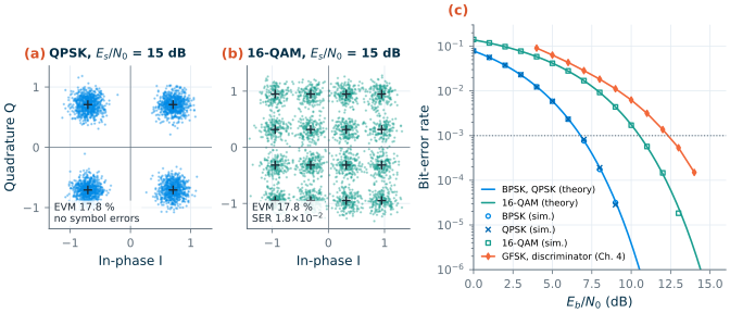
The fair comparison is per bit. With \(E_b/N_0 = (E_s/N_0)/\log_2M\) (Eq. (4.13) of Chapter 4 relates it to the SNR in a bandwidth), BPSK and Gray-coded QPSK have the same bit-error rate,
\[\mathrm{BER} = Q\!\left(\sqrt{2E_b/N_0}\right), \tag{5.3}\]where \(Q\) is the tail of the unit Gaussian distribution. The simulated points of Figure 5.1c fall on it. At a BER of 10−3, QPSK needs an \(E_b/N_0\) of 6.8 dB and 16-QAM 10.5 dB: twice the bits per symbol cost 3.7 dB more energy per bit. BLE’s GFSK, detected with Chapter 4’s simple discriminator, needs 12.3 dB, 5.5 dB more than QPSK.
Why does Bluetooth Low Energy accept that? The answer is power and simplicity, paid for with bandwidth. Pulse shaping (Section 5.2) makes an \(M\)-point modulation occupy \((1+\alpha)R_s\), where \(\alpha\) is the roll-off, so its spectral efficiency is
\[\eta = \frac{\log_2M}{1+\alpha}\ \ \mathrm{b/s/Hz}: \tag{5.4}\]1.48 b/s/Hz for QPSK, 2.96 for 16-QAM and 4.44 for 64-QAM at \(\alpha\) = 0.35. BLE sends 1 Mb/s in a 2 MHz channel, 0.5 b/s/Hz. In exchange, its Gaussian frequency-shift keying (GFSK) carries all the information in the frequency: the envelope is constant, the PA can run saturated, and a receiver can amplify the signal with a limiter and detect it without knowing its carrier phase or amplitude. Each bit shifts the frequency by \(\pm\Delta f\), and the modulation index \(h = 2\Delta f/R_b\) sets how far the phase moves per bit. BLE’s \(h\) = 0.5 gives \(\Delta f\) = 250 kHz: in the I/Q plane, a point running round the unit circle a quarter turn forward or back per bit [184, 65].
What this means for your design
The modulation sets the RF specifications. A constant-envelope signal tolerates a saturated PA and a limiting receiver. QAM and OFDM need a linear chain, and every impairment adds to the EVM like noise: a 16-QAM link at a BER of 10−3 needs \(E_s/N_0\) = 16.5 dB, an EVM of 14.9 % for noise, I/Q imbalance, LO phase noise and PA distortion together.
5.2 Pulse shaping, OFDM and peak-to-average power
Symbols with rectangular pulses have a sinc-shaped spectrum whose sidelobes fall slowly, at 6 dB per octave. QPSK at 1 Mb/s with rectangular pulses keeps only 90.3 % of its power within ±0.5 MHz, and puts −21.7 dBc into the 1 MHz band centred 2 MHz away. At the course radio’s +10 dBm that is −11.7 dBm, far above Bluetooth’s in-band emission limit: −20 dBm at 2 MHz from the carrier and −30 dBm at 3 MHz and beyond, each measured in a 1 MHz band [184].
Nyquist showed how to band-limit pulses without making them interfere: a pulse whose spectrum is odd-symmetric about half the symbol rate passes through zero at every other symbol instant [69]. The raised-cosine pulses are the usual choice. Their spectrum is flat up to \((1-\alpha)R_s/2\) and rolls off as half a cosine period to \((1+\alpha)R_s/2\), which gives Eq. (5.4). The filtering is split into two root-raised-cosine (RRC) filters, one in the transmitter and one, the matched filter, in the receiver. QPSK at 1 Mb/s with \(\alpha\) = 0.35 needs only 578 kHz for 99 % of its power.
GFSK smooths the frequency instead of the amplitude. The bit stream, as a frequency of \(\pm\Delta f\), passes through a Gaussian filter whose bandwidth \(B\) is set by the bandwidth-time product \(BT\) (0.5 for BLE, 0.3 for the GMSK of GSM) [65]:
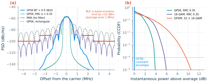
\[\Delta f = \frac{h\,R_b}{2}, \qquad h_G(t) = \sqrt{\frac{2\pi}{\ln 2}}\,B\,\exp\!\left(-\frac{2\pi^2B^2t^2}{\ln 2}\right). \tag{5.5–5.6}\]The phase, the integral of the frequency, is continuous, and the envelope stays constant. Figure 5.2a compares the spectra at 1 Mb/s. GFSK keeps 98.6 % of its power within ±0.5 MHz (99 % within 1031 kHz). The 1 MHz band at 2 MHz receives −65.7 dBc, −55.7 dBm at +10 dBm, 35.7 dB inside the limit; at 3 MHz the GFSK spectrum is below −89 dBm. Without the Gaussian filter, the same phase-continuous FSK (MSK) puts −25.7 dBm at 2 MHz and −33.3 dBm at 3 MHz, only 5.7 and 3.3 dB inside the limits before any PA or LO imperfection adds to them. The filter buys this margin with some inter-symbol interference: each bit’s frequency pulse spreads into its neighbours, one reason GFSK needs more SNR than ideal MSK.
Orthogonal frequency-division multiplexing (OFDM) goes the other way. It splits a fast data stream onto many slow, closely spaced subcarriers, generated together by an inverse FFT [74, 75]; Wi-Fi uses 52 subcarriers 312.5 kHz apart in a 20 MHz channel [186]. Each subcarrier is narrow enough to see a flat channel, which makes OFDM robust against multipath. But the sum of many independent subcarriers is nearly Gaussian, its instantaneous power is exponentially distributed, and it has occasional large peaks. The peak-to-average power ratio is therefore quoted at a probability:
\[\mathrm{PAPR} = \frac{\vert x(t)\vert^2_{peak}}{\langle\vert x(t)\vert^2\rangle}. \tag{5.7}\]Figure 5.2b shows the complementary cumulative distribution (CCDF) of the instantaneous power. The power exceeds its average by more than 3.7 dB for 0.01 % of the time in RRC-filtered QPSK, 5.6 dB in 16-QAM and 9.6 dB in OFDM; an exponential distribution gives \(10\log_{10}(\ln 10^4)\) = 9.6 dB at that probability [83]. GFSK never leaves 0 dB.
A linear PA must pass those peaks without clipping, so its average output must sit a PAPR below its maximum, its back-off. An ideal class-B PA, whose efficiency falls with the square root of its output power, drops from 78.5 % at full power to 26.0 % at 9.6 dB of back-off. Chapter 16 designs PAs and the techniques that recover efficiency in back-off; the course radio’s constant-envelope GFSK lets its PA run at full swing.
5.3 Mixing and the image problem
A mixer multiplies the RF signal by the LO. For two cosines,
\[\cos\omega_{RF}t\cdot\cos\omega_{LO}t = \tfrac{1}{2}\cos(\omega_{RF}-\omega_{LO})t + \tfrac{1}{2}\cos(\omega_{RF}+\omega_{LO})t, \tag{5.8}\]and a low-pass filter keeps the difference, the intermediate frequency (IF). A cosine does not know the sign of its frequency: an input at \(f_{LO} + f_{IF}\) and one at \(f_{LO} - f_{IF}\) both come out at \(f_{IF}\). The second is the image of the first:
\[f_{im} = f_{RF} \mp 2f_{IF}, \tag{5.9}\]with the minus sign for an LO below the wanted channel (low-side injection) and the plus sign for an LO above it [6]. Whatever sits at the image, a signal or only noise, lands on the wanted channel, and no filter after the mixer can separate them. For the course radio, with a 1 MHz IF and the LO below the wanted channel, the image lies 2 MHz below it: the adjacent BLE channel. Even an empty image band costs sensitivity, because the LNA’s noise there folds onto the wanted channel and raises the noise figure by up to 3 dB.
We simulated the problem in ngspice with ideal switches, the simplest model of the passive mixers of Chapter 10. Two double-balanced mixers commutate the RF signal with square-wave LOs at 2.44 GHz, the Q LO a quarter period late; a 20 MHz low-pass filter removes the sum frequency. Six tones of 10 mV, 0.5 to 2 MHz above the LO, form one run, and the same tones below the LO a second run:
* ideal-switch I/Q mixer (mixer_netlist in ch05_architectures.py)
vrf0 r0 0 sin(0 10m 2.441e9)          ; one of six tones: LO + 1 MHz
erp rfp 0 r0 0  0.5                   ; differential RF drive
ern rfn 0 r0 0 -0.5
vli li 0 pulse(-1 1 0 5p 5p 199.9p 409.8p)      ; LO_I, 2.44 GHz
vlq lq 0 pulse(-1 1 102.5p 5p 5p 199.9p 409.8p) ; LO_Q, T/4 late
eli lib 0 li 0 -1
elq lqb 0 lq 0 -1
.model swm sw vt=0 vh=0 ron=1 roff=1e9
s1 rfp ip li  0 swm
s2 rfn in li  0 swm
s3 rfn ip lib 0 swm
s4 rfp in lib 0 swm                   ; s5-s8: qp, qn with lq, lqb
rip ip 0 1k
rin in 0 1k
ei i1 0 ip in 1
ri i1 iout 1k
ci iout 0 8p                          ; 20 MHz low-pass
.tran 1n 6u 0 10p                     ; .options interp: 1 ns grid
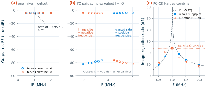
Figure 5.3a shows the I output. Tones above and below the LO come out at the same IF with the same gain, −3.95 dB, the 2/π (−3.92 dB) of a square-wave mixer: one mixer cannot tell them apart. The pair can. In the complex output I − jQ (Figure 5.3b), the tones above the LO appear at positive frequencies and those below at negative frequencies, separated by 75 dB, the numerical floor of the simulation. The quadrature pair keeps the sign of the frequency that a single mixer throws away, and every receiver of Sections 5.5 and 5.6 relies on it. (A square-wave LO also mixes with its odd harmonics, with gains of 1/3 at \(3f_{LO}\) and 1/5 at \(5f_{LO}\): the band filter must keep 7.3 and 12.2 GHz out of the mixer.)
5.4 The heterodyne receiver
The classic answer is to remove the image before the mixer. The heterodyne receiver (Figure 5.4a) puts an image filter between the LNA and the mixer, converts the wanted channel to an IF, selects it there with a channel filter, and converts it again, with an I/Q pair, to baseband [6, 80]. Its two filters pull the IF in opposite directions. The image filter at RF wants the image, \(2f_{IF}\) away, as far as possible; the channel filter wants the IF as low as possible, since selecting a 1 MHz channel at \(f_{IF}\) needs a quality factor of about \(f_{IF}/\)1 MHz.
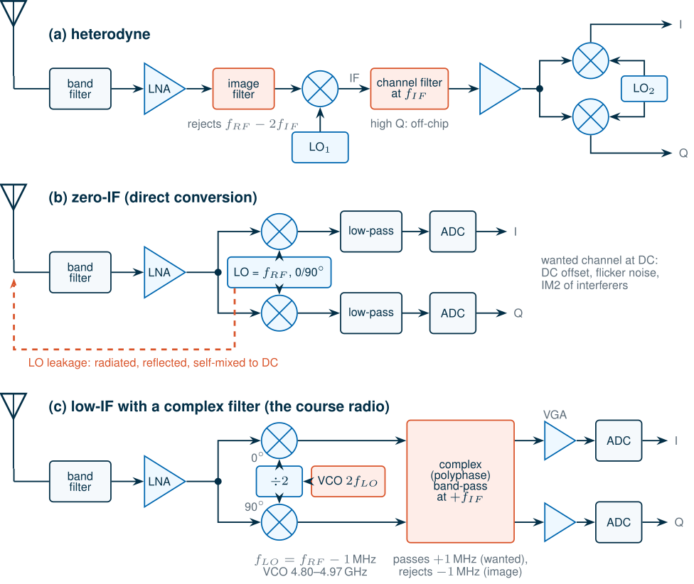
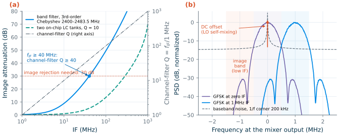
Figure 5.5a puts numbers on the conflict for BLE. Take a third-order Chebyshev band-pass filter for the whole ISM band, 2400–2483.5 MHz, and the lowest channel, 2402 MHz, with the LO below it. Its image is attenuated by 30 dB, the image rejection Section 5.7 asks for, only above an IF of 40 MHz, where the channel filter needs a Q of 40: a surface-acoustic-wave or ceramic filter, off chip. Two on-chip LC tanks with a Q of 10 would need an IF of 285 MHz. At an IF of 1 MHz the band filter attenuates the image by 0.32 dB: nothing. A heterodyne BLE receiver would need external filters, a second LO, and care with the extra spurious responses that every additional mixing step brings, such as the half-IF spur. It gives excellent selectivity, but it is not the architecture of a single-chip, low-cost radio.
5.5 Zero-IF receivers
A zero-IF or direct-conversion receiver puts the LO on the carrier (Figure 5.4b). The image is then the wanted channel’s own mirror: the halves above and below the carrier fold onto each other, but the I/Q pair keeps them apart, and I/Q imbalance only mixes the channel with its own reflection. No image filter is needed, and on-chip low-pass filters select the channel [68, 77]. The price is that the wanted signal now sits at DC, where four problems wait.
DC offsets. The LO leaks to the LNA input through the substrate, the package and the mixer itself, and radiates from the antenna and returns from nearby objects. Mixed with the LO, it becomes a DC voltage indistinguishable from the signal.
Worked example 5.1 · LO self-mixing in a zero-IF receiver
Suppose −60 dBm of LO reaches the LNA input, 60 dB below a 0 dBm LO. In 50 Ω that is 316 µV peak. Through the LNA and mixer of the course budget (16 + 8 = 24 dB of voltage gain) it becomes a DC offset of up to 5.01 mV, depending on its phase. A wanted signal at −90 dBm, 10 µV, arrives at the mixer output as 158.5 µV: the offset is 30 dB larger than the signal, and the 30 dB of baseband gain that follows would turn it into 0.16 V, a large part of the swing of a 1.2 V circuit. Worse, it changes when the antenna’s surroundings move, so a single calibration does not remove it.
The remedy is a high-pass filter or a DC-servo loop, which also cuts the signal near DC. With the Monte Carlo receiver of Section 5.6 at an SNR of 12.3 dB (BER 0.116 %), a first-order high-pass filter in each path raises the BER to 0.133 % at a 5 kHz corner, 0.36 % at 20 kHz and 2.15 % at 50 kHz. At a 1 MHz IF, the same filters leave it at 0.114 %.
Flicker noise. The 1/f noise of the mixer and the baseband circuits (Chapter 4) lands in the channel. With a baseband noise density \(N_0(1 + f_c/\vert f\vert)\) and a channel from \(f_1\) to \(f_2\), the noise in the channel grows by
\[\Delta N = 10\log_{10}\left[1 + \frac{f_c\ln(f_2/f_1)}{f_2 - f_1}\right]. \tag{5.10}\]For a 200 kHz flicker corner, a zero-IF channel from 10 kHz to 500 kHz has 4.14 dB more baseband noise; a low-IF channel from 0.5 to 1.5 MHz only 0.86 dB. With a 1 MHz corner the figures are 9.53 and 3.22 dB. How much of this reaches the receiver’s NF depends on the baseband’s share of the noise budget, which Chapter 4’s cascade puts at about 30 %.
Even-order distortion. Second-order intermodulation turns the envelope of an amplitude-modulated interferer into a low-frequency signal, right where the zero-IF channel sits, which is why IIP2 is the defining linearity number of direct conversion (Chapter 4, Eq. (4.20)). For a modulated interferer of power \(P_B\), the IM2 power in the channel is
\[P_{IM2} = 2P_B - \mathrm{IIP2} + 10\log_{10}(\kappa/2), \tag{5.11}\]where \(\kappa\) is the fraction of the interferer’s envelope-squared fluctuation, \(\vert x\vert^2\) relative to its mean squared, that falls in the channel. Two equal tones give \(\kappa\) = 0.5 at their difference frequency and Eq. (5.11) reduces to Eq. (4.19). A low IF does not escape this: a 20 MHz-wide Wi-Fi signal has envelope content from DC to 16 MHz, including 0.5–1.5 MHz.
Worked example 5.2 · IIP2 for a Wi-Fi interferer
The OFDM signal of Figure 5.2b, as a Wi-Fi interferer, has \(\kappa\) = 0.11 in the course radio’s IF band (from its simulated envelope spectrum), so \(10\log_{10}(\kappa/2)\) = −12.6 dB. Let the receiver keep its sensitivity with a Wi-Fi interferer at −40 dBm: the IM2 must stay 6 dB below the noise floor of −107.9 dBm in 1 MHz (which raises the noise by 1 dB). Then \(\mathrm{IIP2} \ge 2(-40) - (-113.9) - 12.6\) = +21.3 dBm at the antenna. The mixer, behind 14 dB of gain (filter and LNA), produces most of the IM2 (the LNA’s low-frequency products are blocked by the coupling to the mixer), so its own IIP2 must reach +35.3 dBm. At −30 dBm the receiver would need +41.3 dBm: every 10 dB of interferer costs 20 dB of IIP2.
LO leakage and self-image. The leaking LO also radiates from the antenna at the channel frequency, and I/Q imbalance folds the channel onto itself, which degrades the EVM of QAM signals.
Figure 5.5b summarizes: at zero IF the GFSK spectrum sits on top of the DC offset and the flicker noise; at 1 MHz it lies above both, at the price of an image band at −1 MHz.
5.6 Low-IF and image-reject receivers
A low-IF receiver offsets the LO from the carrier by about one channel bandwidth [76, 79]. It keeps the integration of the zero-IF receiver, with no external filters and on-chip channel selection, while moving the signal away from DC. Its image is the neighbouring channel, \(2f_{IF}\) away, too close for any RF filter. The image must therefore be rejected by the I/Q processing that Figure 5.3b introduced, with one of three structures.
Hartley. Shift the Q signal by a further 90° and add it to I (Figure 5.6a): the wanted signal’s two copies add and the image’s cancel; the difference gives the image alone [70]. The simplest 90° shift is an RC low-pass filter in one path and a CR high-pass filter in the other. Their phases differ by exactly 90° at every frequency, but their gains are equal only at \(f_0 = 1/2\pi RC\); the gain ratio \(f/f_0\) sets the rejection:
\[\mathrm{IRR}(f) = \left(\frac{1 + f/f_0}{1 - f/f_0}\right)^2. \tag{5.12}\]The image-rejection ratio (IRR) is the gain to the wanted signal divided by the gain with which the image reaches the wanted output. Figure 5.3c adds such a combiner, with \(f_0\) = 1.00 MHz, to the ngspice mixers. With an ideal LO the simulated IRR follows Eq. (5.12): 9.5 dB at 0.5 MHz, 16.9 dB at 0.75 MHz, 19.1 dB at 1.25 MHz, 14.0 dB at 1.5 MHz, and 77.7 dB at 1 MHz, where only the numerical floor limits it. A GFSK channel at a 1 MHz IF spans 0.5–1.5 MHz, so a single RC–CR stage is not enough; practical designs cascade several stages with staggered corners, a polyphase filter [81].
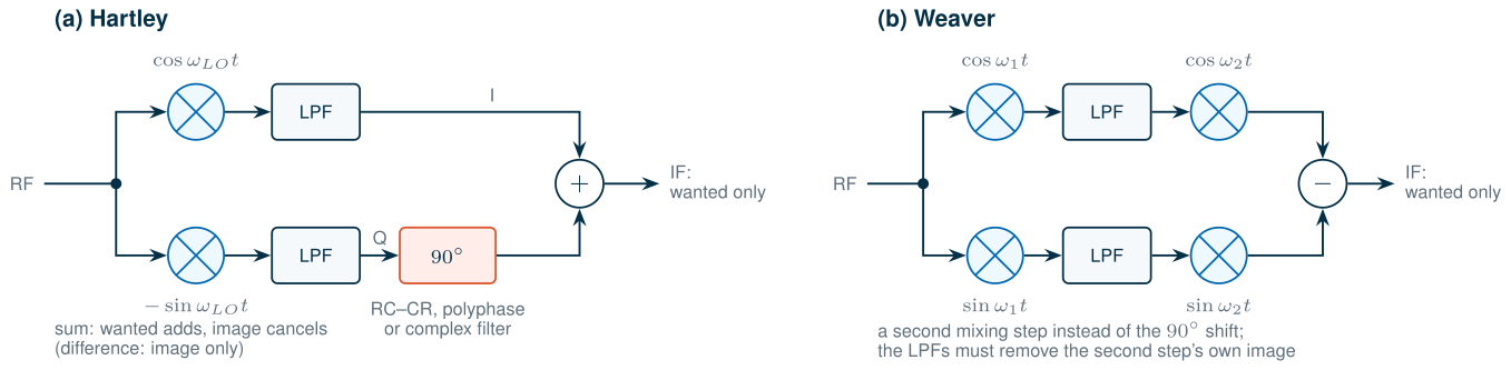
Weaver. Replace the 90° shift by a second quadrature mixing step (Figure 5.6b) [73]. Mixers are easier to match over a band than RC networks, but the second step has an image of its own, which the low-pass filters between the steps must remove.
Complex filters. The course radio takes a third route. A filter that acts on I + jQ as one complex signal can have different responses at positive and negative frequencies. Take a low-pass prototype and shift it to \(+f_{IF}\), replacing \(s\) by \(s - j\omega_{IF}\): in hardware, two identical real filters whose integrators are cross-coupled between the I and Q paths [79]. The result selects the channel at +1 MHz and rejects the image at −1 MHz in one block (Figure 5.4c). Our model of it is the fourth-order Butterworth low-pass filter of Chapter 4, with a 1 MHz noise bandwidth (cut-off 487.2 kHz), shifted to +1 MHz. It attenuates the image band by 50.8 dB.
To see the image at work, we simulated a low-IF receiver in the time domain. The RF signal is real, with the carrier scaled from 2.44 GHz to 24 MHz (sampled at 192 MHz): the image problem depends only on the offsets from the LO, and the scaled carrier keeps the LO’s sum products far from the band. A wanted GFSK channel sits 1 MHz above the LO and an image channel, 9 dB stronger as in BLE’s image test, 1 MHz below; two real multipliers with cosine and sine LOs and identical fourth-order low-pass filters produce I and Q. Figure 5.7a shows the I output alone: the image lands on top of the wanted channel, 9 dB above it, and no filter can take it away. In the complex output (Figure 5.7b), the image sits at −1 MHz, where the complex filter removes it. With 1 dB of gain error and 5° of phase error between the paths, however, a mirror of the image, 22.8 dB below it, appears at +1 MHz, inside the wanted channel, where no filter can reach it. The I/Q accuracy, not the filter, sets the image rejection.
5.7 I/Q imbalance and the image-rejection ratio
Let the quadrature LO have a gain error \(\varepsilon\) and a phase error \(\theta\): \(LO_I = 2\cos\omega_{LO}t\) and \(LO_Q = -2(1+\varepsilon)\sin(\omega_{LO}t + \theta)\). For an input whose complex envelope relative to the LO is \(z\), the complex output after the low-pass filters is
\[y = K_1z + K_2z^*, \qquad K_1 = \frac{1 + (1+\varepsilon)e^{-j\theta}}{2}, \qquad K_2 = \frac{1 - (1+\varepsilon)e^{j\theta}}{2}. \tag{5.13}\]A wanted signal at \(+f_{IF}\) reaches \(+f_{IF}\) through \(K_1\); an image at \(-f_{IF}\) reaches \(-f_{IF}\) through \(K_1\) and, conjugated, \(+f_{IF}\) through \(K_2\). The ratio is the image rejection:
Key equation · Image-rejection ratio of a quadrature receiver
\[\mathrm{IRR} = \frac{\vert K_1\vert^2}{\vert K_2\vert^2} = \frac{1 + 2(1+\varepsilon)\cos\theta + (1+\varepsilon)^2}{1 - 2(1+\varepsilon)\cos\theta + (1+\varepsilon)^2} \approx \frac{4}{\varepsilon^2 + \theta^2} \tag{5.14}\]with \(\theta\) in radians; the approximation holds for small errors. One degree of phase error alone limits the IRR to 41.2 dB.
Derivation · The output of an imbalanced quadrature mixer
Write the input as \(x(t) = \mathrm{Re}\{z\,e^{j\omega_{LO}t}\} = \tfrac{1}{2}(z\,e^{j\omega_{LO}t} + z^*e^{-j\omega_{LO}t})\). Multiplying by \(2\cos\omega_{LO}t\) and keeping the low-frequency part gives \(I = \mathrm{Re}\{z\} = (z + z^*)/2\). Multiplying by \(-2(1+\varepsilon)\sin(\omega_{LO}t + \theta)\) gives \(Q = (1+\varepsilon)\,\mathrm{Im}\{z\,e^{-j\theta}\} = (1+\varepsilon)(z\,e^{-j\theta} - z^*e^{j\theta})/2j\). Then
\[I + jQ = \frac{z + z^*}{2} + (1+\varepsilon)\frac{z\,e^{-j\theta} - z^*e^{j\theta}}{2},\]which collects into Eq. (5.13). For \(\varepsilon = \theta = 0\), \(K_1 = 1\) and \(K_2 = 0\). For small errors, \(\vert K_1\vert^2 \approx 1\) and \(\vert K_2\vert^2 \approx (\varepsilon^2 + \theta^2)/4\), the approximation in Eq. (5.14).
Figure 5.7c checks Eq. (5.14) against the passband simulation, with single tones at the LO ± 1 MHz and gain errors of 0 to 2 dB and phase errors of 0.25° to 10°. They agree to within 10−10 dB: for ideal multipliers and identical filters, Eq. (5.14) is exact. The ngspice switch mixers of Figure 5.3c, with the Q LO 3° late and 1 dB more gain in the Q path, give 23.97 dB against 23.99 dB from Eq. (5.14). Gain and phase errors trade against each other: 0.5 dB and 1° give 30.4 dB, 0.2 dB and 2° give 33.6 dB, 1 dB and 5° only 22.8 dB.
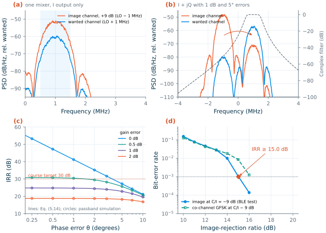
How much IRR does BLE need? Its image test puts an interferer 9 dB above a wanted signal at −67 dBm, 3 dB above the standard’s reference sensitivity of −70 dBm [184]. A complex-envelope version of the receiver (16 MHz sampling, the I/Q model of Eq. (5.13), the complex filter and Chapter 4’s discriminator) answers by Monte Carlo. With perfect I/Q it reproduces Chapter 4’s sensitivity: 12.4 dB of SNR for a BER of 10−3, against 12.3 dB. With the image at C/I = −9 dB (Figure 5.7d), the BER reaches 10−3 at an IRR of 15.0 dB. The image’s mirror behaves like a co-channel GFSK interferer, which the discriminator tolerates down to a C/I of 7.0 dB: 7.0 + 9 = 16.0 dB, within a decibel of the image result.
Common pitfall · Treating interference as noise
If the mirrored image is treated as noise, the receiver seems to need 12.3 + 9 = 21.3 dB of IRR. The simulation needs 15.0 dB. A GFSK interferer has a constant envelope and a bounded effect on the phase, so the discriminator ignores it until it is strong enough to flip a decision, and then the error rate climbs steeply (Figure 5.7d). Noise-equivalent budgets are a safe first guess for interference, but the receiver’s real tolerance comes from a simulation with the real signals.
The course radio asks for an IRR of 30 dB, 15.0 dB more than the image test needs. The margin covers what the test does not: production spread (the mismatch is random, so the IRR must hold for nearly every chip), images stronger than the test’s, and wanted signals near the course’s sensitivity instead of at −67 dBm. The errors come from the divide-by-two that makes the quadrature LO, the mixers and the complex filter. The allocation is a gain error of at most 0.2 dB and a phase error of at most 2° for the whole I/Q path, which gives 33.6 dB, without calibration (Chapters 10 and 13).
5.8 Transmitter architectures
A transmitter has the opposite job: turn I and Q into RF at the right power, inside the emission mask. Three structures cover most radios (Figure 5.8).
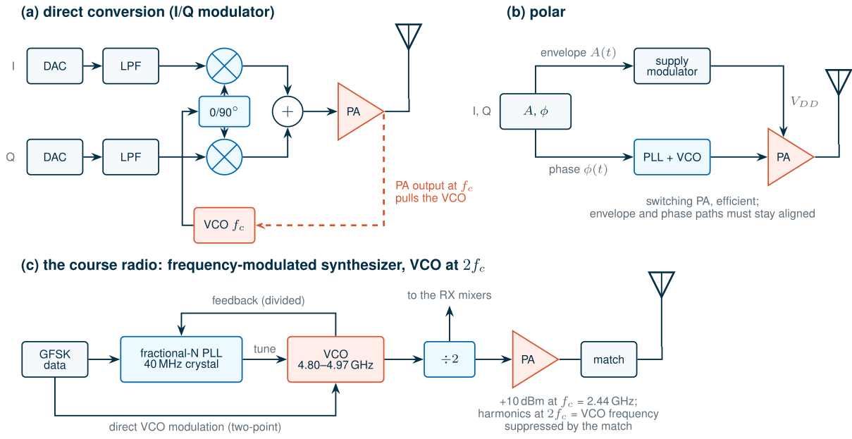
Direct conversion. An I/Q modulator mixes the baseband I and Q up to the carrier, and a PA amplifies the sum (Figure 5.8a). It handles any modulation, which is why it dominates in multi-standard radios [6]. Its impairments mirror those of the zero-IF receiver: LO leakage appears as a carrier in the middle of the channel, and I/Q imbalance produces an unwanted sideband with the suppression of Eq. (5.14). The serious problem is injection pulling: the PA’s large output sits at the VCO’s frequency and couples back into it through the substrate, the supply and the inductors’ magnetic fields. An oscillator perturbed by a signal near its frequency locks to it within Adler’s lock range [71, 82]
\[\omega_L = \frac{\omega_0}{2Q}\,\frac{I_{inj}}{I_{osc}}, \tag{5.15}\]and is pulled, its spectrum corrupted, when the injection lies just outside it.
Worked example 5.3 · How little coupling it takes to pull a VCO
A VCO at 2.44 GHz with a tank Q of 10 receives a fraction of the PA’s output that is 40 dB (a factor of 100 in current) below its own oscillation. By Eq. (5.15) the lock range is \(f_L\) = 2.44 GHz/20 × 0.01 = 1.22 MHz, wider than the whole modulated spectrum of a BLE signal. A coupling of −40 dB between two blocks on the same die is easily reached, so the VCO of a direct-conversion transmitter must not run at the PA’s frequency.
The usual remedy is to place the VCO at a different frequency: twice the carrier with a divide-by-two, or 2/3 or 4/3 of it with an extra mixer. A two-step transmitter achieves the same by modulating at an IF and converting to RF with a second LO, which needs a filter for the unwanted sideband.
Polar. Split the signal into its envelope \(A(t)\) and phase \(\phi(t)\) (Figure 5.8b) [72]. The phase modulates a PLL or a phase modulator, which drives an efficient switching PA; the envelope sets the PA’s supply. The two paths must stay aligned in time and the envelope path must be wide: for OFDM, several times the channel bandwidth. For a constant-envelope signal, \(A\) is constant and the polar transmitter reduces to its phase path.
The course radio. That phase path is the course transmitter (Figure 5.8c). The GFSK data steers the fractional-N divider of the synthesizer, and the synthesizer’s output, divided by two, drives the PA. The PLL’s bandwidth, typically a few hundred kilohertz, is narrower than the 1 Mb/s modulation, so the data must either be pre-emphasized digitally [78] or applied at two points, the divider and the VCO’s tuning input, two-point modulation, with matched gains (Chapter 14). There is no I/Q modulator, no DAC at RF and no linear PA. The VCO runs at 4.80–4.97 GHz, twice the carrier, for three reasons:
- Quadrature for the receiver. A divide-by-two made of two latches produces I and Q 90° apart, with an accuracy set by the VCO’s duty cycle and the latches’ matching, not by an RC network: the 2° of Section 5.7 (Chapter 13).
- No pulling at the fundamental. The PA’s +10 dBm at 2.44 GHz is half the VCO frequency. Its second harmonic does fall on the VCO frequency, but the output network suppresses it (Chapter 16), and because it is derived from the VCO itself it is coherent with it: a static phase shift that the PLL corrects, not a spur.
- A smaller tank. At 4.9 GHz the same tank capacitance needs a quarter of the inductance, and small spirals in SG13G2’s thick top metals reach their best Q at several gigahertz (Chapter 7).
The cost is a VCO and a divider running at 4.9 GHz. Dividing by two lowers the phase noise by \(20\log_{10}2\) = 6.0 dB, so the VCO’s specification is 6 dB higher than the LO’s, which is the same oscillator quality at twice the frequency.
5.9 The course radio’s architecture and link budget
The architecture and the IF
Table 5.1 sums up the comparison for a BLE receiver.
Table 5.1. Receiver architectures for the course radio (numbers from this chapter's simulations).
| Heterodyne | Zero-IF | Low-IF (1 MHz) | |
|---|---|---|---|
| Image | filtered at RF: IF ≥ 40 MHz for 30 dB | the channel’s own mirror | adjacent channel, rejected by I/Q accuracy |
| Channel selection | off-chip filter, Q ≥ 40 | on-chip low-pass | on-chip complex band-pass |
| DC offset, high-pass filter | none | BER 0.116 → 0.36 % with a 20 kHz high-pass | none (0.114 %) |
| Flicker penalty, 200 kHz corner | none | 4.14 dB | 0.86 dB |
| IM2 of modulated interferers | out of band | in band | in band (IIP2 ≥ +21.3 dBm for −40 dBm Wi-Fi) |
| LOs, external parts | two LOs, SAW/ceramic filters | one LO | one LO |
The course radio is a low-IF receiver with quadrature down-conversion and a complex channel filter. The IF of 1 MHz is the lowest at which the GFSK channel (99 % of its power within 1031 kHz) clears the region near DC: at 1 MHz it spans 0.5–1.5 MHz, above a DC-blocking high-pass corner of tens of kilohertz and above most of the flicker noise. A higher IF would widen the complex filter and the ADCs, which costs power, and move the image to channels where BLE allows stronger interferers. BLE tests the receiver’s image frequency, wherever it falls, at C/I = −9 dB, a concession to low-IF receivers, and its image ± 1 MHz at −15 dB [184]; with a 1 MHz IF the image is the adjacent channel below. The LO may sit on either side of the wanted channel, whichever image is quieter, so the VCO must cover 2 × (2401–2481 MHz) = 4.802–4.962 GHz, inside the specified 4.80–4.97 GHz.
From the standard to the specifications
Table 5.2 turns BLE’s requirements into the course radio’s specifications. For each, the left column is what the standard itself demands, the right what the course asks, which is tighter because the course receiver aims at −90 dBm instead of the standard’s −70 dBm.
Table 5.2. Receiver requirements from Bluetooth Low Energy (1M PHY, BER 0.1 %) and the course radio's specifications. SNRmin = 12.3 dB (Chapter 4), noise bandwidth 1 MHz. BLE's 0.1 % holds for receivers whose longest supported payload is 37 bytes, a packet error rate of 30.8 %; a receiver that accepts 255-byte payloads must reach 0.017 %, about the same packet error rate.
| Quantity | BLE test → requirement | Course specification | Course budget |
|---|---|---|---|
| Sensitivity, NF | −70 dBm → NF ≤ 31.7 dB | −90 dBm → NF ≤ 11.7 dB; spec 8 dB | NF 6.06 dB, −95.6 dBm |
| IIP3, Eq. (5.16) | two −50 dBm interferers, wanted −64 dBm → ≥ −36.9 dBm | ≥ −15 dBm (interferers up to −35.4 dBm) | −12.7 dBm |
| Blocking | −35 dBm at 2399 and 2484 MHz | 1 dB desensitization above −35 dBm | ≈ −25.3 dBm |
| IIP2 (antenna) | — (CW and GFSK interferers have no IM2 in the channel) | ≥ +21.3 dBm: Wi-Fi at −40 dBm, Worked example 5.2 | mixer ≥ +35.3 dBm |
| Image rejection | image at C/I = −9 dB → IRR ≥ 15.0 dB | ≥ 30 dB | 33.6 dB (0.2 dB, 2°) |
| LO phase noise at 3 MHz | −40 dBm interferer, wanted −67 dBm → ≤ −99.3 dBc/Hz | −40 dBm interferer, wanted −87 dBm → ≤ −119.9 dBc/Hz | −110 dBc/Hz at 1 MHz: −119.5 dBc/Hz |
Noise and linearity. Chapter 4 derived the noise-figure limit, 11.7 dB for −90 dBm, and the illustrative cascade, NF 6.06 dB and IIP3 −12.7 dBm, which this chapter adopts. BLE’s intermodulation test applies two interferers of −50 dBm, a CW tone and a modulated BLE signal 3, 4 or 5 MHz apart (a receiver must pass one of the three spacings), whose third-order product falls on a wanted signal at −64 dBm, 6 dB above the reference sensitivity [184]. The product must stay \(\mathrm{SNR}_{min}\) below the wanted signal:
\[\mathrm{IIP3} \ge \frac{3P_I - (P_w - \mathrm{SNR}_{min})}{2}, \tag{5.16}\]−36.9 dBm. The course’s −15 dBm handles interferer pairs up to −35.4 dBm, 14.6 dB stronger than the test. It also covers blocking: by Chapter 4’s rules, the receiver’s IP1dB is about IIP3 − 9.6 dB = −22.3 dBm, and a blocker desensitizes it by 1 dB about 3 dB lower, near −25.3 dBm, 9.7 dB above BLE’s −35 dBm blockers at 2399 and 2484 MHz, which the band filter barely attenuates.
Reciprocal mixing and the LO phase noise. A strong interferer \(\Delta f\) away from the wanted channel mixes with the LO’s phase noise \(\mathcal{L}(\Delta f)\) (Chapter 11), which spreads it over the wanted channel: reciprocal mixing. In a bandwidth \(B\) the spread power is
Key equation · Reciprocal mixing and the phase noise it requires
\[P_{RM} = P_B + \mathcal{L}(\Delta f) + 10\log_{10}B \tag{5.17}\] \[\mathcal{L}(\Delta f) \le C/I - \mathrm{SNR}_{min} - 10\log_{10}B \tag{5.18}\]\(C/I\) is the wanted power over the interferer power in dB; the offset that matters is the interferer’s distance from the wanted channel, whatever the IF.
We checked Eq. (5.17) with the complex-envelope receiver: a CW blocker at 2, 3 and 5 MHz from the wanted channel, multiplied by an LO with a synthesized phase noise (within 0.11 dB of the requested \(\mathcal{L}(f)\)), through the complex filter. The in-channel power agrees with Eq. (5.17) within 0.35 dB, and with the exact integral of \(\mathcal{L}(f)\) over the filter’s response within 0.02 dB (Figure 5.9). BLE’s interferers [184] then set mild requirements: −89.3 dBc/Hz at 2 MHz (C/I = −17 dB), −99.3 dBc/Hz at 3 MHz and beyond (C/I = −27 dB), and −104.3 dBc/Hz for the −35 dBm CW blockers at 2399 and 2484 MHz, 27 and 58 MHz from the 2426 MHz channel on which BLE tests out-of-band blocking. The −30 dBm blockers below 2000 MHz and above 3000 MHz ask for −109.3 dBc/Hz, but at least 426 MHz away, where the LO is near its noise floor.
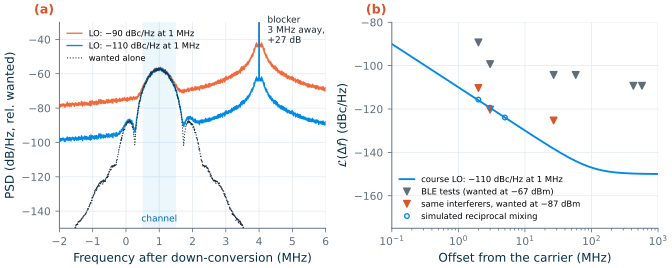
Those requirements assume a wanted signal at −67 dBm. The course receiver should keep its interference tolerance near its own sensitivity: with the wanted signal 3 dB above −90 dBm, at −87 dBm, and the same −40 dBm interferer 3 MHz away, the reciprocal mixing must leave 12.3 dB of SINR together with the receiver’s noise. That asks for −119.9 dBc/Hz at 3 MHz with the budget’s NF of 6.06 dB (−120.3 dBc/Hz at the 8 dB specification, −119.3 dBc/Hz if the receiver were noiseless). With a skirt of −20 dB/decade this is −110 dBc/Hz at 1 MHz, the course specification, which gives −119.5 dBc/Hz at 3 MHz: the course case sets it, with no margin to spare. At the VCO, at twice the frequency, it becomes −104.0 dBc/Hz at 1 MHz. The same LO is harmless elsewhere: its integrated phase error from 10 kHz to 8 MHz is 1.11° rms, its rms frequency error in the channel 2.94 kHz against GFSK’s 250 kHz deviation, and in the transmitter its phase noise puts −46.0 dBm into the band 2 MHz away (limit −20 dBm) and −49.5 dBm at 3 MHz (limit −30 dBm).
The block budget
Table 5.3 is the budget the block chapters design to; Chapter 19 checks the designed blocks against it.
Table 5.3. Block specifications of the course radio's receiver and synthesizer (cascade as in Chapter 4, Table 4.2; tt, 27 °C).
| Block | Gain (dB) | NF (dB) | IIP3 (dBm) | Other specifications | Designed in |
|---|---|---|---|---|---|
| Band filter + T/R switch | −2 | 2 | +40 | 2400–2483.5 MHz; out-of-band rejection | Ch. 8, 19 |
| LNA | +16 | 2.5 | −6 | S11 ≤ −10 dB across the band; 1.2 V | Ch. 9 |
| I/Q mixer (with TIA) | +8 | 12 | +4 | IIP2 ≥ +35.3 dBm; I/Q path (with LO and filter): gain error ≤ 0.2 dB, phase error ≤ 2° | Ch. 10 |
| LO: VCO ÷ 2 | — | — | — | VCO 4.802–4.962 GHz; L ≤ −110 dBc/Hz at 1 MHz at the LO (≤ −104.0 dBc/Hz at the VCO) | Ch. 11–14 |
| Complex filter + VGA | +30 | 20 | +14 | 4th-order Butterworth, 1 MHz noise bandwidth at +1 MHz; image band rejected by 50.8 dB | sibling course; Ch. 19 |
| Receiver | +52 | 6.06 | −12.7 | sensitivity −95.6 dBm; IRR 33.6 dB | Ch. 19 |
Checking the budget
A budget built from separate requirements can still miss an interaction: an interferer that is both near the image and strong enough for reciprocal mixing, say. So we ran every BLE interference test through the complex-envelope receiver with the allocated impairments at once: I/Q errors of 0.2 dB and 2°, the course LO’s phase noise, the complex filter, noise for NF = 6.06 dB, and the wanted signal at −67 dBm. For each interferer, a GFSK signal at the test’s offset, the interference was raised in 3 dB steps (6 × 104 bits each) until the BER passed 10−3 (Table 5.4).
Table 5.4. BLE interference tests (wanted −67 dBm, GFSK interferers) against the behavioural course receiver: the C/I at which the BER reaches 0.1 %. Negative C/I: interferer stronger than the wanted signal. Offsets from the wanted channel; the LO is 1 MHz below it. Where two of BLE's requirements apply to one offset (−1 MHz is also the image + 1 MHz, −2 MHz also the 2 MHz neighbour, −3 MHz also ≥ 3 MHz away), the more relaxed one applies [184]. BLE also excuses five spurious-response channels at least 2 MHz away, other than the image and image ± 1 MHz, if they meet C/I = −17 dB.
| Interferer | BLE requirement C/I (dB) | Simulated tolerance C/I (dB) | Margin (dB) |
|---|---|---|---|
| Co-channel | 21 | 6.7 | 14.3 |
| +1 MHz | 15 | −5.9 | 20.9 |
| −1 MHz (lands at DC) | 15 | −5.5 | 20.5 |
| +2 MHz | −17 | −36.8 | 19.8 |
| −2 MHz (image) | −9 | −26.4 | 17.4 |
| +3 MHz | −27 | −46.4 | 19.4 |
| −3 MHz (image − 1 MHz) | −15 | −38.5 | 23.5 |
| +4 MHz | −27 | −49.5 | 22.5 |
| −4 MHz | −27 | −49.4 | 22.4 |
Every test passes with at least 14.3 dB of margin. The image test’s 17.4 dB is the IRR of 33.6 dB less the 15.0 dB the image needs, as Section 5.7 predicts. At +3 MHz the limit is no longer the filter but the reciprocal mixing: an interferer 46.4 dB above the wanted signal spreads, through −119.5 dBc/Hz, about as much power into the channel as the discriminator tolerates. The model leaves out the ADC, the transmitter’s carrier offset (BLE allows ±150 kHz, initial offset and drift within the packet together [184]), the real filter’s group delay and the circuits’ own nonlinearity; Chapter 19 adds them with the designed blocks. The carrier offset turns out to matter: at ±150 kHz the 1 MHz filter of Table 5.3 cuts into the shifted GFSK spectrum and loses 4.9 dB of sensitivity, so Section 19.2 widens it to a 1.4 MHz noise bandwidth, at the cost of some adjacent-channel margin.
Try it · The architecture script
Every number in this chapter comes from
tools/figs/ch05_architectures.py:python3 tools/figs/ch05_architectures.pyredraws everything from the cached simulations in about a minute, and--resimreruns them all (about ten minutes, one of them the ngspice mixers). Three experiments: (1) Incompliance_part, set the LO to −100 dBc/Hz at 1 MHz (the argument ofphase_noise) and runcompliance --resim: which BLE test fails first, and does its margin follow Eq. (5.18)? (2) Inreceiver, lower the complex filter’sorderfrom 4 to 2 and runcompliance --resim: which adjacent-channel margins shrink, and why does the image test hardly move? (3) Inmixer_netlist, change the Hartley resistorRCHby 5 % and rerunmixer --resim: by how much does the 1 MHz IRR fall, and how does that compare with Eq. (5.14) for a 5 % gain error?
- A digital modulation is a constellation in the I/Q plane. Denser constellations raise the spectral efficiency (QPSK 1.48, 16-QAM 2.96 b/s/Hz at α = 0.35) but need more Eb/N0 (6.8 and 10.5 dB for 10−3); BLE’s GFSK needs 12.3 dB but has a constant envelope, a saturated PA and a simple receiver.
- Pulse shaping keeps the spectrum in its channel: BLE’s Gaussian filter puts −55.7 dBm at 2 MHz for +10 dBm, against a −20 dBm limit. OFDM peaks 9.6 dB above its average (at 10−4), which forces a linear PA into back-off; GFSK has 0 dB.
- A mixer cannot tell the image from the wanted signal; an I/Q pair can. The heterodyne filters the image (IF ≥ 40 MHz for BLE, off-chip filters), the zero-IF receiver avoids it but meets DC offsets, flicker noise and IM2, and the low-IF receiver rejects it with I/Q processing.
- The IRR of a quadrature receiver is about 4/(ε² + θ²), exactly Eq. (5.14) for ideal mixers. BLE’s image test needs 15.0 dB; the course asks for 30 dB and allocates 0.2 dB and 2° (33.6 dB).
- The course VCO runs at 2fc: the divide-by-two gives the quadrature LO, the PA does not pull the VCO at its fundamental, and the VCO may have 6 dB more phase noise than the LO (−104 dBc/Hz at 1 MHz).
- The course budget, NF 6.06 dB, IIP3 −12.7 dBm, IIP2 +21.3 dBm, IRR 33.6 dB and −110 dBc/Hz at 1 MHz, passes every BLE interference test with at least 14.3 dB of margin in a behavioural simulation; the phase noise is set by receiving near the course’s sensitivity, not by the standard.
Further reading
- B. Razavi, RF Microelectronics [6], Chapters 3 and 4: modulation, the image problem, and heterodyne, direct-conversion and image-reject transceivers, with many more variants than this chapter shows.
- A. A. Abidi, “Direct-conversion radio transceivers for digital communications” [68], and B. Razavi, “Design considerations for direct-conversion receivers” [77]: why zero-IF came back, and what it costs.
- J. Crols and M. Steyaert, “Low-IF topologies for high-performance analog front ends of fully integrated receivers” [79]: complex signals and polyphase filters, the theory behind the course radio’s receiver; S. Mirabbasi and K. Martin [80] for a short tour of all the architectures.
- J. G. Proakis and M. Salehi, Digital Communications [19]: modulation, detection and error rates in depth.
- B. Razavi, “A study of injection locking and pulling in oscillators” [82]: Adler’s equation applied to the pulling of VCOs by PAs.