Lab 5
The I/Q Passive Mixer
Take Chapter 10's 25 % current-mode mixer apart and put it back together: the switch and its fit, the NAND gates that make the four LO phases, the conversion gain in Xyce, the noise figure from a harmonic transfer matrix, and the linearity and I/Q accuracy with one switch 1 % too wide.
- Characterize an SG13G2 RF switch in Xyce and fit the behavioural conductance that the noise analysis needs, with SciPy.
- Generate four 25 % LO phases with NAND gates and inverters at 2.4 GHz, and measure their duty cycle, edges, overlap and power.
- Simulate the mixer’s conversion gain, input impedance and I/Q accuracy at RF = 220 Ω, and know when Xyce’s time step limits them.
- Compute the SSB noise figure of a periodically switched circuit with Chapter 10’s periodic small-signal module, and split it into its sources.
- Measure IIP3, IIP2 and the I/Q gain and phase errors with a deliberate 1 % switch mismatch.
Contents
| Lab 5 at a glance | |
|---|---|
| Goal | The course mixer’s switch, LO, gain, noise figure, linearity and I/Q errors from your own runs, against Chapter 10. |
| Chapters | Chapter 10 (Sections 10.2, 10.3, 10.5, 10.7 and 10.8; Eqs. (10.3)–(10.5)); Chapter 2 for transient and periodic analyses |
| Time | 3 hours |
| Files | tools/labs/lab5/: mixer_lab.py; it imports tools/figs/ch10_mixers.py (netlists and measurements) and tools/figs/_ch10_lptv.py (periodic small-signal noise) |
| Run time | switch and lo about 8 s together; mixer 2–5 min (Xyce, 1.2 µs of a 2.4 GHz LO); noise a few seconds |
Hand calculation
The course mixer (Figure 10.1) has four switches of 64 µm with \(R_{sw}\) = 20.6 Ω and a gate capacitance of 79.6 fF each, driven at \(f_{LO}\) = 2.400 GHz from 1.2 V, and two TIAs with \(R_F\) = 220 Ω. Before you simulate:
- Conversion gain. Evaluate Eq. (10.3), \(G = (2\sqrt2/\pi)\,R_F/(R_S + R_{sw})\), in dB. Then replace \(R_{sw}\) by the input resistance that Chapter 10 simulated, 28.4 Ω, and evaluate it again.
- LO power. Evaluate Eq. (10.4), \(P_{LO} \approx \tfrac{4}{3}\cdot4\,C_gV_{DD}^2f_{LO}\).
- Noise figure. Evaluate the four terms of Eq. (10.5) at \(R_F\) = 220 Ω with T = 300.15 K, \(T_0\) = 290 K and an op-amp noise of \(e_n\) = 1.29 nV/√Hz, and add them up. Which term is largest?
Steps
Work in tools/labs/lab5. Inside the container run the commands as shown; from your own computer, put ../common/iic.sh in front of each (Lab 0). Each step writes its Xyce netlist into out/, runs Xyce -plugin …/Xyce_Plugin_PSP103_VA.so on it there, and prints what it measured. Xyce runs these SG13G2 transients many times faster than ngspice’s OSDI model (Section 10.8), which is why this lab uses it throughout.
-
The switch.
cd /foss/designs/rfic-design/tools/labs/lab5 python3 mixer_lab.py switch # from your computer: ../common/iic.sh python3 mixer_lab.py switchout/mix_switch_dc.cirsweeps the gate of one 8 µm cell (with its 40 Ω gate resistance) from 0 to 1.2 V with 10 mV across the channel at \(V_{CM}\) = 0.3 V;out/mix_switch_ac.cirputs the four switches of the mixer on one RF node, once with one switch on and once with all off, and measures the node’s capacitance at 2.4 GHz. The script fits \(g(V_G) = ks\ln\!\left(1 + e^{(V_G - V_t)/s}\right)\) to the conductance above 0.8 V withscipy.optimize.curve_fit[178], weighting each point by its own value so that the fit minimizes the relative error. It prints \(R_{on}W\), the switch’s \(R_{sw}\), the gate voltage at which it reaches 5 % of its on-conductance, the fit and its worst error. The noise step uses the fit and the mean capacitance. -
The 25 % LO.
python3 mixer_lab.py loout/mix_lo.ciris the LO generator of Figure 10.3a: ideal 50 % I and Q square waves (30 ps edges, as from the divider of Chapter 13) drive four NAND gates (8/8 µm) with their inputs stacked so that every pulse starts at the top input, each followed by an inverter (12/24 µm) that drives one switch of the mixer. Read theX…lines of one NAND and find which input sits at the top of the nMOS stack. The script measures, over the last ten of twelve LO periods, the duty cycle at \(V_{DD}/2\) and above the switch’s turn-on voltage from step 1, the 10–90 % edges, the time per edge during which two switches conduct together, and the supply power. -
The mixer.
python3 mixer_lab.py mixer # 2-5 minutesout/mix_rf220.cirholds three copies of the course mixer with \(R_F\) = 220 Ω on one ideal four-phase LO (pulses 0 to 1.2 V, 25 ps edges): copyawith a 3 mV tone at LO + 1 MHz, copiescanddwith two tones at LO + 3 and LO + 5 MHz at −16 and −4 dBm per tone, and with switch 0 one per cent wider than the others. The TIAs are behavioural, as in the chapter: an op-amp with 40 dB of gain and one pole at 10 MHz. After 0.2 µs of settling, the script takes a 1 µs record on a 25 ps grid and Fourier-transforms it. From copyait gets the conversion gain against the available source voltage, the current conversion gain, the input impedance at LO + 1 MHz, and the gain and phase of Q against I; from copiescanddthe IM3 at 1 MHz and the IM2 at 2 MHz, referred to the input through the gain of copya, and the I/Q errors with the mismatch.Look at the
.tranline: its last field limits Xyce’s time step to 2 ps (MAXSTEPin the script). Without it, Xyce’s step control lets the gain wander by ±0.03 dB and the I/Q phase by about 0.1° between runs of slightly different netlists, which is larger than the errors this step is meant to measure. Try it once: delete the field, rerun Xyce with the command the script printed, and analyse withpython3 mixer_lab.py mixer --nosim. -
The noise figure.
python3 mixer_lab.py noiseNeither ngspice nor Xyce has a periodic noise analysis (Section 2.6), so this step solves the periodically time-varying circuit directly, by the periodic small-signal method [32], with
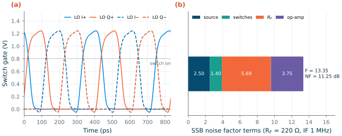
analyse()oftools/figs/_ch10_lptv.py. It samples one LO period of the four gate voltages (lo_gate()of Chapter 10, the same trapezoids as the pulse sources of step 3), turns them into four conductances \(g_k(t)\) with your fit from step 1, and builds the harmonic transfer matrix of the circuit for the sidebands \(f_{IF} + nf_{LO}\), \(n\) = −40…40: the source, the coupling capacitor, the RF node with its 173 fF, the four switches, \(C_{in}\) and the two behavioural TIAs. Each switch’s thermal noise is cyclostationary, with a correlation between sidebands set by the Fourier coefficients of \(g_k(t)\). The step prints the SSB noise figure at a 1 MHz IF and its four terms (source, switches, \(R_F\), op-amp), the noise figure after ideal image rejection, the same analysis with ideal switches of \(R_{sw}\) that switch at \(V_{DD}/2\), and Eq. (10.5) with \(R_{sw}\) and with the simulated input resistance of step 3. -
Everything at once.
python3 mixer_lab.py allruns the four steps, stores the checkpoint numbers inlab_numbers.jsonand draws Figure L5.1 intoout/.
Checkpoint
Table L5.1. Lab 5 results (SG13G2, tt, 27 °C; LO 2.400 GHz; RF = 220 Ω; noise at a 1 MHz IF, 290 K source). Tolerance: ±1 in the last digit shown, except where stated.
| Quantity | Lab 5 | Chapter 10 |
|---|---|---|
| Hand calculation: Eq. (10.3) with \(R_{sw}\) / with 28.4 Ω | 8.96 / 8.05 dB | 8.96 dB |
| Hand calculation: Eq. (10.4); Eq. (10.5) at 220 Ω | 1.47 mW; 10.6 dB (terms 2.47, 1.05, 4.63, 3.33) | 1.47 mW; 10.6 dB |
| Switch: \(R_{on}W\), \(R_{sw}\) (64 µm), turn-on voltage | 1315 Ω·µm, 20.6 Ω, 0.803 V | 1320 Ω·µm (3 digits), 20.6 Ω, 0.803 V |
| Switch fit: \(V_t\), \(s\), worst error above 0.8 V | 0.854 V, 54.7 mV, 4.2 % | 0.855 V, 55 mV, 4.2 % |
| RF-node capacitance of the four switches: one on / all off / mean | 182 / 163 / 173 fF | 182 / 163 / 173 fF |
| LO chain: duty cycle at \(V_{DD}/2\) / above turn-on | 29.6 / 26.4 % | 29.6 / 26.4 % |
| LO chain: rise, fall (10–90 %); overlap per edge (±0.2 ps) | 40.7, 36.0 ps; 5.5 ps | 40.7, 36.0 ps; 5.65 ps |
| LO chain: supply power | 2.73 mW | 2.73 mW |
| Conversion gain; current conversion gain | +8.02 dB; −6.91 dB | +8.02 dB; −6.93 dB |
| Input impedance at LO + 1 MHz (±0.3 Ω) | 28.6 − j3.1 Ω | 28.4 − j3.0 Ω |
| I/Q gain and phase, matched switches (±0.015 dB, ±0.01°) | 0.000 dB, 90.00° | 0.013 dB, 89.99° |
| SSB noise figure (periodic small-signal) | 11.25 dB | 11.25 dB |
| Noise factor terms: source, switches, \(R_F\), op-amp | 2.50, 1.40, 5.69, 3.75 | 2.50, 1.40, 5.68, 3.75 |
| NF after ideal image rejection; gain in the periodic analysis | 8.24 dB; 7.92 dB | 8.24 dB; 7.93 dB |
| The same with ideal switches: NF, gain | 10.62 dB, 8.80 dB | 10.63 dB, 8.79 dB |
| Eq. (10.5) with the simulated input resistance | 11.29 dB (28.6 Ω) | 11.23 dB (28 Ω) |
| Two tones at −16 dBm: IIP3; compression | +10.0 dBm; −0.06 dB | +9.9 dBm; −0.05 dB |
| Two tones at −4 dBm: IIP3; compression | +9.3 dBm; −1.14 dB | +9.3 dBm; −1.14 dB |
| IIP2 with the 1 % mismatch, at −4 dBm (±1 dB) | +55.2 dBm | +56.0 dBm |
| I/Q errors with the 1 % mismatch, at −16 dBm (±0.01°) | −0.015 dB, −0.009° | −0.016 dB, −0.001° |
The switch, the LO chain and the noise figure reproduce Chapter 10 within the stated tolerances (the chapter rounds \(R_{on}W\) to three digits). The transient numbers agree within tolerances that come from Xyce’s time-step control rather than from the circuit. With the 2 ps step limit, this lab’s matched I and Q are in quadrature to 0.0002 dB and 0.001°; the chapter’s run, without the limit but with more devices in the same netlist, left 0.013 dB and 0.009°. Both are numerical floors, far below the 0.2 dB and 2° of the receiver’s budget. For the same reason the I/Q phase error with the mismatch, below 0.01° in both runs, is a bound rather than a measurement. The IIP2 is a checkpoint only at −4 dBm: at −16 dBm the IM2 product lies about 80 dB below the fundamental, near the floor of the transient, and this run gives +59.8 dBm where the chapter’s gave +67.1 dBm. The chapter quotes the −4 dBm value.
Questions
- The LO chain draws 2.73 mW, 1.86 times Eq. (10.4). Eq. (10.4) counts the switch gates and a third more for the buffers. Where does the rest go? (Look at the edges of step 2 and at what an inverter does while its input crosses the middle.)
- With ideal switches the periodic analysis agrees with Eq. (10.5) to 0.03 dB; with the fitted switches it is 0.63 dB higher and the gain is 0.87 dB lower. Use the input impedance to explain both, and say why every noise term grows when the gain falls.
- At 2.4 GHz a 25 % pulse lasts 104 ps. The duty cycle at \(V_{DD}/2\) is 29.6 %, yet above the turn-on voltage it is only 26.4 %, with 5.5 ps per edge in which two switches conduct. Which of the two numbers decides the conversion gain, and what would a gap with no switch on cost?
- One switch 1 % wider limits IIP2 to about +55 dBm, yet moves the I/Q phase by less than 0.01°. Why does a width mismatch hurt the even-order product so much more than the quadrature?
- The IIP3 hardly changes between −16 and −4 dBm although the gain is compressed by 1.1 dB at −4 dBm. What does that say about the order of the nonlinearity, and where in the circuit would you look for it?
Extension
Drive the mixer from the LO chain instead of the ideal pulses. In step_mixer() of mixer_lab.py, replace C10.lo_sources("q", 0.25) by C10.lo_inputs() + ["vddq vddq 0 1.2"] + C10.lo_chain("q", "vddq"): the chain then drives the gate nodes g0q…g3q that the mixers use. Rerun mixer and compare the gain and the input impedance with the ideal LO; Chapter 10 found +8.20 dB and 26.1 Ω, because the slower edges let two switches conduct together for longer. Then set RF = 200.0 at the top of the script and rerun mixer noise with the ideal LO, to reproduce the chapter’s first design (+7.18 dB, 11.57 dB). Which buys more noise figure per milliwatt, a larger \(R_F\) or faster LO edges?