Chapter 12
PLL Dynamics and Phase Noise
A phase-locked loop does not just multiply a crystal's frequency: it decides, offset by offset, whose noise reaches the antenna. This chapter follows every noise source of a charge-pump PLL to its output, finds the loop bandwidth that minimizes the jitter, estimates the reference spurs, checks when the continuous-time model stops being true, and closes the course synthesizer's phase-noise budget with the VCO that Chapter 11 simulated: a 400 kHz loop with a third-order filter that meets −110 dBc/Hz at 1 MHz with 3.0 dB to spare, and 451 fs of rms jitter.
- Design a third-order passive loop filter for a chosen loop bandwidth and phase margin, and explain what its extra pole buys and costs.
- Derive the transfer function from each noise source of a charge-pump PLL (reference, divider, charge pump, loop-filter resistors, VCO) to the output phase.
- Compute the integrated jitter of a PLL and find the loop bandwidth that minimizes it.
- Estimate reference spurs from charge-pump leakage and current mismatch, by hand and from the Fourier series of the charge-pump current.
- Recognize when the sampled nature of the phase detector invalidates the continuous-time model, and build a phase-noise budget that the next chapter can extend.
Contents
12.1 Where the analog course stopped
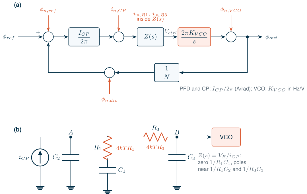
The PLL chapter of The Art of Analog IC Design built a complete charge-pump PLL [4]: a phase-frequency detector (PFD) that turns the time between a reference edge and a divided VCO edge into an UP or DN pulse, a charge pump that turns the pulse into charge, an R–C1–C2 loop filter, a ring VCO and a divider. It derived Gardner’s linear model [135], in which the PFD and charge pump are a gain \(I_{CP}/2\pi\) (amperes per radian), the filter an impedance \(Z(s)\), the VCO an integrator \(2\pi K_{VCO}/s\) and the divider a gain \(1/N\). The loop gain is
\[G(s) = \frac{I_{CP}K_{VCO}}{N}\,\frac{Z(s)}{s}, \tag{12.1}\]with \(K_{VCO}\) in Hz/V. It designed the filter for a loop bandwidth \(f_u\) (where \(\vert G\vert = 1\)) and a phase margin, noted that the loop is really sampled once per reference period, and simulated the loop locking. It stopped at noise: it showed that the output follows the reference inside the loop bandwidth and the VCO outside, but did not ask how much noise each block contributes.
That is the question a radio asks. Chapter 5 set the course LO’s phase noise at −110 dBc/Hz at 1 MHz, −104 dBc/Hz at the VCO, which runs at twice the LO. Chapter 11 built a VCO that meets this on its own, and Chapter 13 a divider chain. This chapter closes the loop around them (Figure 12.1a): a 40 MHz crystal, \(N\) = 122 (VCO at 4.880 GHz, LO at 2.440 GHz, the middle of the band), the Chapter 11 VCO with \(K_{VCO}\) = 131 MHz/V (the centre of the 103–167 MHz/V that the loop sees after Chapter 11’s band calibration, from its transients), and a charge pump and filter designed here. Fractional division, which the course needs for its 2 MHz channel spacing, and its quantization noise belong to Chapter 14; everything here is integer-N, and Chapter 14 adds its noise to the budget of Section 12.7.
12.2 Higher-order loop filters
Why add a pole
In lock, the charge pump does not deliver a smooth current. Once per reference period it delivers a short pulse (Section 12.5), and the filter turns that pulse train into a ripple on the control voltage at \(f_{ref}\) and its harmonics. The ripple frequency-modulates the VCO and appears as reference spurs 40 MHz either side of the carrier, inside the 2.4 GHz ISM band. The second-order filter attenuates the ripple only by the single pole of \(C_2\). A third-order filter (Figure 12.1b) adds a low-pass section \(R_3\)–\(C_3\) between the filter and the VCO [22, 11]. Its transimpedance has the same zero and integrator, and two poles:
\[Z(s) = \frac{1 + sT_2}{s\,C_{tot}\,(1 + sT_1)(1 + sT_3)}, \qquad T_2 = R_1C_1, \quad C_{tot} = C_1 + C_2 + C_3. \tag{12.2}\]\(T_1\) is roughly \(R_1C_2\) and \(T_3\) roughly \(R_3C_3\), but the two sections load each other (in the course filter below, \(1/2\pi R_1C_2\) = 2.76 MHz while the first pole sits at 1.75 MHz), so the exact poles follow from the components by multiplying out the network (the script solves the nodal equations). The extra pole costs phase at the loop bandwidth:
\[\mathrm{PM} = \arctan\omega_uT_2 - \arctan\omega_uT_1 - \arctan\omega_uT_3. \tag{12.3}\]Design equations
The phase margin is largest when the loop crosses unity at the peak of Eq. (12.3). Because \(\arctan x + \arctan y \approx \arctan(x + y)\) for the small angles of the poles, the two poles act like one with time constant \(T_1 + T_3\), and the second-order recipe of the sibling course (zero a factor \(b\) below \(\omega_u\), pole a factor \(b\) above) carries over:
\[T_2 \approx \frac{b}{\omega_u}, \qquad T_1 + T_3 \approx \frac{1}{b\,\omega_u}, \qquad \mathrm{PM} \approx \arctan b - \arctan\frac{1}{b}. \tag{12.4}\]The total capacitance then follows from \(\vert G(j\omega_u)\vert = 1\) with Eqs. (12.1) and (12.2):
\[C_{tot} = \frac{I_{CP}K_{VCO}}{N\,\omega_u^2}\,\frac{\sqrt{1 + \omega_u^2T_2^2}}{\sqrt{(1 + \omega_u^2T_1^2)(1 + \omega_u^2T_3^2)}}. \tag{12.5}\]Two choices remain: how to split \(T_1 + T_3\), and one component value, since the five components must satisfy only four conditions (\(T_2\), \(C_{tot}\) and the two poles). Moving the third pole down towards the first attenuates the ripple more (the product \(T_1T_3\) is largest for an even split), but the interaction of the two sections then forces a small \(C_3\) and a large \(R_3\), and \(R_3\) is noisy (Section 12.3): with \(T_3/T_1\) = 0.5 the course loop has a passive solution only for \(C_3\) up to 0.27 pF, which needs \(R_3\) = 181 kΩ. We take \(T_3 = 0.15\,T_1\) and fix \(C_3\) at 1.9 % of \(C_{tot}\), about 1.2 pF, large enough to swamp the VCO’s tuning-input capacitance. The script solves Eq. (12.3) exactly for the phase peak at \(\omega_u\) and then the components in closed form (after Banerjee [22]).
Worked example 12.1 · The course loop filter
Take \(f_u\) = 400 kHz (Section 12.4 explains the choice), PM = 60°, \(I_{CP}\) = 100 µA (Section 12.7), \(K_{VCO}\) = 131 MHz/V and \(N\) = 122. Eq. (12.4) gives \(b\) = 3.73, a zero at 400/3.73 ≈ 107 kHz and \(T_1 + T_3\) placing the combined pole near 1.5 MHz. The sibling course’s Eq. (23.8), \(R \approx N\omega_u/(I_{CP}K_{VCO})\), predicts \(R_1\) ≈ 23.4 kΩ. The exact designs:
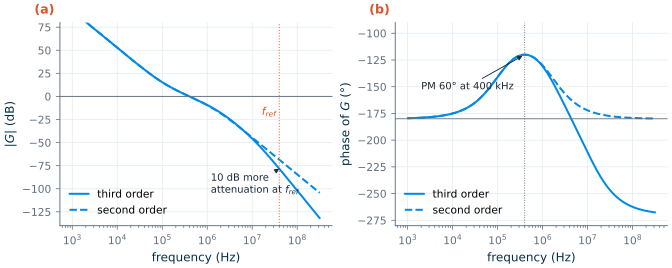
Second order Third order R1, C1 25.2 kΩ, 59.0 pF 24.5 kΩ, 60.0 pF C2 4.56 pF 2.35 pF R3, C3 — 19.0 kΩ, 1.21 pF Zero; poles 107 kHz; 1.49 MHz 108 kHz; 1.75 MHz and 11.6 MHz Total capacitance 63.5 pF 63.5 pF \(\vert Z\vert\) at 40 MHz 872 Ω 282 Ω Both filters reach \(f_u\) = 400 kHz with PM = 60.0° (Eq. (12.4) predicts 60.0°). The 63.5 pF is 0.0423 mm² of MIM capacitance at about 1.5 fF/µm² [191], the largest single item of the synthesizer’s area. The third-order filter cuts the impedance at the reference frequency by 9.8 dB for no extra capacitance.
\(K_{VCO}\) is the number to get right first, and the right number is the one the loop sees, not the VCO’s average. The first version of this design used Chapter 11’s small-signal estimate, 108 MHz/V; the second, the transients’ mean over 0–1.2 V at code 8, 96.9 MHz/V. But after band calibration (Section 11.8) the loop settles where the tuning curve is steep, and sees 103–167 MHz/V over every channel and corner. The design takes the geometric centre, 131 MHz/V, so that the loop gain stays within ±2.1 dB of its design value at both ends. The filter designed for 96.9 MHz/V (\(R_1\) = 33.2 kΩ, \(C_{tot}\) = 46.9 pF) would cross unity at 524 kHz at the centre of that range and 648 kHz at its top, where the phase margin falls to 57.0°. Since \(C_{tot} \propto I_{CP}K_{VCO}\) and \(R_1 \propto 1/(I_{CP}K_{VCO})\) (Eqs. 12.4–12.5), re-solving grows the capacitors by 35 % and shrinks the resistors by 26 %, and the poles and the zero stay where they were. The alternative, a charge-pump current scaled down by the same factor to keep \(I_{CP}K_{VCO}\) constant, would keep the filter but cost more noise: the charge pump’s referred noise grows as \(1/I_{CP}\) (Eq. 12.7), and the resistors’ with \(K_{VCO}^2\) at a fixed \(R\).
Figure 12.2 shows the two loop gains. They coincide up to about 2 MHz; above it the third-order loop falls at 60 dB per decade instead of 40, and its phase keeps falling. The extra pole cost nothing in phase margin here, because the design re-centred the zero and the first pole around \(f_u\); it costs a slightly smaller \(C_2\) and a second noisy resistor. Over the calibrated range, 103–167 MHz/V, the filter is fixed and \(f_u\) moves from 323 kHz to 496 kHz, while the phase margin stays at 59.4° at both ends: the peak of Eq. (12.3) is broad.
12.3 Noise transfer functions of a PLL
One loop, five transfer functions
Each noise source of Figure 12.1a enters the loop at a different point, and the loop treats each differently [11, 21]. Write \(H = G/(1+G)\) for the closed-loop response. Then, working round the loop:
- Reference and divider. Phase noise at the PFD input, from the crystal or from the divider’s output edges, is indistinguishable from a real phase change of the reference. The loop makes the output follow it, multiplied by \(N\):
- Charge pump. A noise current \(i_{n,CP}\) at the charge-pump output is equivalent to a phase error \(2\pi i_{n,CP}/I_{CP}\) at the PFD:
- Loop-filter resistors. The thermal noise of \(R_1\) or \(R_3\), written as a current \(i_{n,R}\) (with \(\overline{i_{n,R}^2} = 4kT/R\) per hertz) across the resistor, produces a voltage at the VCO input through a transimpedance \(Z_n(s)\) of the filter; the VCO integrates it into phase, and the loop corrects what it can:
- VCO. The loop measures the VCO’s phase and corrects it, so its noise is high-passed:
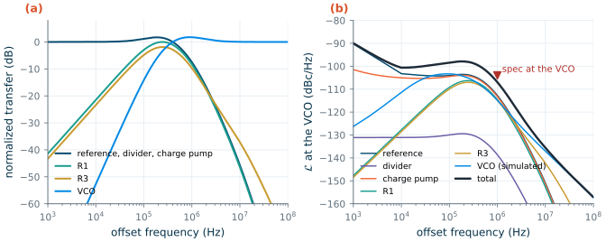
Figure 12.4a plots the shapes. Everything before the filter (reference, divider, charge pump) shares the low-pass \(NH\): flat at \(N^2\) = 41.7 dB inside the loop bandwidth, with a peak of 1.72 dB near \(f_u\) (the price of 60° of phase margin), and falling at 40–60 dB per decade above. The resistors are band-pass: below the zero the loop corrects their noise, above the poles the capacitors short it. The VCO is high-pass: suppressed at 40 dB per decade inside the loop bandwidth, slightly amplified around \(f_u\), untouched above. \(R_3\) differs from \(R_1\) at high offsets: \(C_2\) shunts \(R_1\)’s noise above the first pole, but \(R_3\)’s noise reaches the VCO directly until the \(R_3C_3\) pole at 6.95 MHz.
The reference and the divider
The crystal is a commercial part: a 2.0 × 1.6 mm, 40 MHz TCXO (temperature-compensated crystal oscillator) whose typical single-sideband phase noise is −132 dBc/Hz at 1 kHz, −145 dBc/Hz at 10 kHz and −147 dBc/Hz at 100 kHz [208]. The datasheet stops at 100 kHz; we assume the noise stays at −147 dBc/Hz beyond, the usual floor of a clipped-sine TCXO output. Multiplied by \(N^2\) this floor becomes −105.3 dBc/Hz at the VCO, −111.3 dBc/Hz at the LO: on its own, the reference already sits only 1.3 dB below the LO’s specification at 1 MHz. Inside the loop bandwidth the reference alone keeps the course radio from getting much better than that; a crystal with a lower floor, or a higher reference frequency (smaller \(N\)), is the remedy.
The divider’s noise enters at the same point. Chapter 13 estimated 40.5 fs of edge jitter for its CML divide-by-two and asked for the counters’ 40 MHz output to be retimed [144]. We assume the retimed edge carries the jitter of two such stages (the retiming flip-flop and the PFD), √2 × 40.5 = 57.3 fs. By Chapter 13’s Eq. (13.9), referred to the VCO, that is −131.1 dBc/Hz in band, negligible; without retiming, 1 ps would give −106.3 dBc/Hz, as much as the reference.
The charge pump
The charge pump is the one block of the loop simulated at transistor level in this chapter (ngspice [194], SG13G2 typical models): an NMOS and a PMOS current mirror of long devices, each with a minimum-length switch in series, mirrored from ideal 100 µA references.
* SG13G2 charge pump, both sources on (as during the PFD reset), output held at 0.6 V
IREFN vdd nbn 100u
XMN0 nbn nbn 0 0 sg13_lv_nmos W=32u L=4u ng=4     ; DN mirror (gm/ID = 7.17)
XMN1 dnd nbn 0 0 sg13_lv_nmos W=32u L=4u ng=4
XMNS outn vdd dnd 0 sg13_lv_nmos W=4u L=0.13u ng=2 ; DN switch, on
IREFP pbp 0 100u
XMP0 pbp pbp vdd vdd sg13_lv_pmos W=128u L=4u ng=8 ; UP mirror (gm/ID = 6.82)
XMP1 upd pbp vdd vdd sg13_lv_pmos W=128u L=4u ng=8
XMPS outp 0 upd vdd sg13_lv_pmos W=8u L=0.13u ng=2 ; UP switch, on
VSN out outn 0
VSP outp out 0
VOUT out 0 0.6 ac 1
HM nm 0 VOUT 1                                     ; output noise current as a voltage
.control
dc VOUT 0.1 1.1 0.01
noise v(nm) VOUT dec 20 100 1e9
.endc
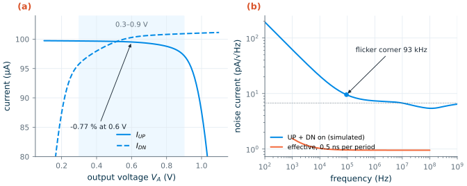
The devices have \(V_{DS,sat}\) ≈ 0.25 V, so each source needs about 0.3 V of headroom including its switch. Figure 12.3a shows the two currents against the output voltage. At 0.6 V they are 99.52 µA (UP) and 100.3 µA (DN), a mismatch of −0.77 %; across 0.3–0.9 V, the useful control range, the mismatch grows to 4.0 % at the ends, because each mirror’s output then sits far from its diode’s drain voltage. (A replica amplifier that copies the output voltage onto the reference branches would flatten this [11].)
Figure 12.3b is the noise analysis with both sources on: 6.74 pA/√Hz of white noise, which is what \(\sqrt{4kT(2g_{m,n} + 2g_{m,p})}\) gives (6.81 pA/√Hz, with each mirror’s diode noise copied to the output), and flicker noise below a corner of 93.1 kHz despite the 4 µm channels. The noise analysis is a snapshot with the sources permanently on. In lock they conduct only during the PFD’s reset pulse, which we take as 0.5 ns per 25 ns period (an assumption: long enough for the sources to settle and avoid a dead zone, short enough to keep the noise down). A switched noise current is a noise current multiplied by a pulse train of duty cycle \(d\); white noise folds from every harmonic of the pulse train and is scaled by \(d\), while slow flicker noise only sees the pulse train’s average and is scaled by \(d^2\) [11, 21]:
\[S_{i,eff}(f) \approx d\,S_{i,white} + d^2\,S_{i,1/f}(f), \qquad d = t_{on}f_{ref}. \tag{12.10}\]With \(d\) = 2.0 %, Eq. (12.7) puts the charge pump at −105.7 dBc/Hz at the VCO in band, level with the reference. Both scale in the obvious way: the charge pump’s contribution falls by 3 dB for each doubling of \(I_{CP}\) (Section 12.7) and rises with the on-time, which Chapter 14’s fractional divider will lengthen.
All sources together
Figure 12.4b adds everything up for the course loop, at the VCO. The VCO is the one Chapter 11 simulated with every noise source (node ISFs and frozen device noise, code 8): −89.2 dBc/Hz at 100 kHz and −116.7 dBc/Hz at 1 MHz, an equivalent noise factor F = 3.71 and a 1/f³ corner of 254 kHz, scaled by 0.02 dB from 4.868 to 4.880 GHz. Four regions appear:
- below 10 kHz, the crystal’s own close-in noise, multiplied by \(N^2\);
- from 10 kHz to about 400 kHz, the in-band plateau: reference (−104.1 dBc/Hz at 100 kHz) and charge pump (−104.5 dBc/Hz), with the resistors 5–6 dB lower, and the VCO’s 1/f³ region rising to their level (−103.4 dBc/Hz at 100 kHz);
- around \(f_u\) and up to a few megahertz, everything at once: at 1 MHz the VCO gives −114.9 dBc/Hz, the reference −112.8, the charge pump −113.2 and the two resistors −114.6 and −114.9 dBc/Hz, for a total of −107.0 dBc/Hz;
- above a few megahertz, the free-running VCO, with \(R_3\) a distant second.
At 1 MHz the total is 3.0 dB below the VCO’s specification of −104 dBc/Hz. No single source dominates, which is typical of a well-balanced loop: each block was given roughly the same share. (Before Chapter 11 simulated the VCO, this budget used its first estimate: a noise factor between 2 and 5 for the 1/f² region and an assumed 1/f³ corner of 1 MHz, Leeson’s empirical form of Eq. (11.8) [120]. At the pessimistic end, F = 5, the VCO’s contribution at 1 MHz would be −110.6 dBc/Hz and the total −105.9 dBc/Hz; the simulation removes that uncertainty, and Section 12.7 keeps the bracket only as a sensitivity check.)
12.4 Integrated jitter and the optimum bandwidth
A single phase-noise number at 1 MHz says how much a blocker 1 MHz away spreads into the wanted channel (reciprocal mixing, Chapter 5). The demodulator, the ADC clocked by the synthesizer, and the transmitted signal’s error-vector magnitude see the integrated noise instead: the rms phase error and its timing equivalent, the jitter,
\[\phi_{rms} = \sqrt{2\int_{f_1}^{f_2}\mathcal{L}(f)\,df}, \qquad \sigma_t = \frac{\phi_{rms}}{2\pi f_0}, \tag{12.11}\]where the factor 2 turns the single-sideband \(\mathcal{L}\) back into the phase spectrum. We integrate from 10 kHz to 10 MHz at the LO. (Dividing by two halves \(\phi_{rms}\) and the frequency together, so the jitter in seconds is the same at the VCO and at the LO, apart from the divide-by-two’s own floor of −158.1 dBc/Hz from Chapter 13, which adds 3.6 fs.)
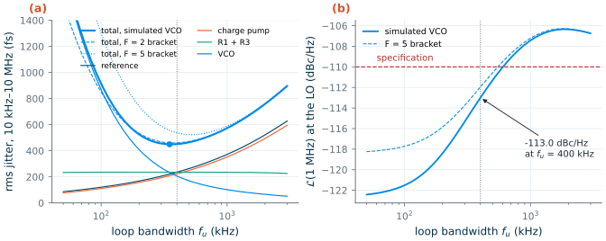
The loop bandwidth trades the two halves of Figure 12.4b against each other. A narrower loop lets more of the VCO’s large close-in noise through; a wider loop passes the in-band plateau out to higher offsets. The jitter is lowest near the bandwidth where the in-band plateau meets the free-running VCO’s noise [21, 11]. Figure 12.5a shows the sweep: for each \(f_u\) the script redesigns the filter with the rules of Section 12.2 (same PM, pole ratio and \(I_{CP}\)) and integrates Eq. (12.11). With the simulated VCO the optimum is 350 kHz (449 fs). The minimum is shallow: 400 kHz costs 2 fs, while a 50 kHz loop would give 1780 fs and a 3 MHz loop 897 fs. A noisier VCO wants a wider loop: Chapter 11’s earlier bracket would have put the optimum at 387 kHz (460 fs) for F = 2 and 527 kHz (523 fs) for F = 5, the dashed curves of Figure 12.5a.
The specification at 1 MHz adds a second constraint (Figure 12.5b). As \(f_u\) approaches 1 MHz, the in-band plateau (−111.3 dBc/Hz at the LO from the reference alone) and the peaking of \(NH\) arrive at the 1 MHz offset. The course loop meets −110 dBc/Hz up to \(f_u\) ≈ 583 kHz (527 kHz with the F = 5 estimate). We choose 400 kHz: within a few femtoseconds of the jitter optimum, with −113.0 dBc/Hz at 1 MHz, room for the spread of \(K_{VCO}\) after calibration (which moves \(f_u\) between 323 and 496 kHz), and a bandwidth a hundred times below \(f_{ref}\), which keeps the sampled-loop effects of Section 12.6 away. It is also the “few hundred kilohertz” Chapter 5 anticipated: too narrow for the 1 Mb/s GFSK data to pass through the divider alone, hence two-point modulation (Chapter 14).
12.5 Reference spurs
From ripple to spur
In lock the average charge-pump current is zero, but its waveform is not: a short pulse each period, whose fundamental \(I_1\) (peak amplitude) flows into the filter and leaves a ripple \(V_1 = I_1\vert Z(j2\pi f_{ref})\vert\) on the control voltage. A sinusoidal ripple frequency-modulates the VCO with a deviation \(K_{VCO}V_1\); for a small modulation index each sideband is half the index [11]:
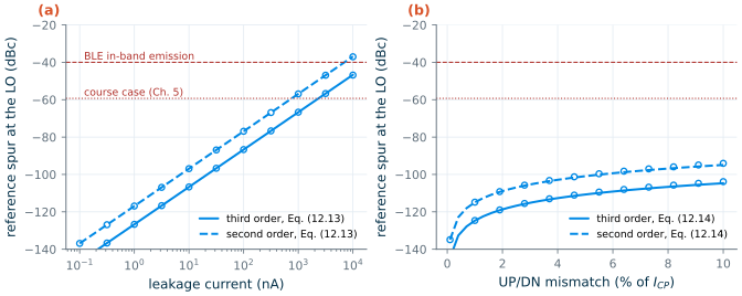
\[\frac{P_{spur}}{P_c} = 20\log_{10}\frac{K_{VCO}V_1}{2f_{ref}}. \tag{12.12}\]Two mechanisms give the fundamental. A leakage current \(I_{leak}\) at the filter node (junctions of the switches, gate leakage of MOS capacitors or of the varactor) must be replaced every period, so the loop settles with a phase offset at which the charge pump delivers a pulse of charge \(I_{leak}/f_{ref}\). A narrow pulse train of average \(I_{leak}\) has a fundamental of twice the average:
\[I_1 \approx 2I_{leak}. \tag{12.13}\]An UP/DN mismatch \(\Delta I\) leaves a net charge \(\Delta I\,t_{rst}\) during each reset pulse, which the loop cancels with an equal and opposite charge just before it (a static phase offset). The two packets are about \(t_{rst}/2\) apart, so their fundamentals nearly cancel; the residue is
\[I_1 \approx 2\pi f_{ref}^2\,\Delta I\,t_{rst}^2. \tag{12.14}\]A timing skew \(\delta t\) between the UP and DN switches acts like a mismatch with \(\Delta I\,t_{rst} = I_{CP}\,\delta t\). Divided by two for the LO, the spur falls by 6 dB.
How large are they?
Figure 12.6 compares Eqs. (12.13) and (12.14) with the exact Fourier series of the charge-pump current in lock (rectangular pulses with the offset that makes the average zero, as the script builds it), through the second- and third-order filters of Worked example 12.1. The hand formulas match the exact series within 1 dB. For 1 nA of leakage the spur at the LO is −127 dBc with the third-order filter and −117 dBc with the second-order filter; for the 4 % mismatch that the simulated charge pump reaches at the edges of its range (Figure 12.3a), −112 and −103 dBc. The third pole buys its 9.8 dB at every point.
What do we need? A spur 40 MHz away on the LO mixes an interferer 40 MHz away onto the wanted channel, and on the transmitter it is an emission 40 MHz from the carrier. Bluetooth’s in-band emission limit of −30 dBm at 3 MHz and beyond [184] allows −40 dBc at +10 dBm. Chapter 5’s harder course case, a −40 dBm interferer with the wanted signal at −87 dBm and SNRmin = 12.3 dB, asks for −59.3 dBc. The leakage would have to reach 2340 nA (third order) or 758 nA (second order) to violate even that. On these mechanisms alone, the course synthesizer’s reference spurs are no concern.
That conclusion is narrower than it looks. Eqs. (12.13) and (12.14) describe a charge pump with ideal edges. Real charge pumps also inject the switches’ channel charge and couple the switching edges through their gate–drain capacitance, the reference and the PFD pulse couple into the VCO’s supply, substrate and tuning line, and in a fractional-N loop the divider’s changing modulus moves the pulse every period (Chapter 14). Those effects, which are layout-dependent, usually set the spur level of a real synthesizer; the extra pole of the third-order filter attenuates whatever reaches the filter node, which is why it is worth having.
12.6 Sampled-loop effects
The z-domain view
Gardner’s linear model averages the charge-pump current over each reference period. The real PFD acts only once per period: it measures the phase error at the reference edge and delivers one pulse. Between edges the filter and the VCO evolve on their own. That is a sampled system, and it is exactly described by a recursion from one edge to the next [135, 136]. Collect the three capacitor voltages and the VCO phase in a state vector \(\mathbf{x}\), with continuous-time dynamics \(\dot{\mathbf{x}} = A\mathbf{x}\) between pulses. If the pulses are short compared with the period, each is a charge \(I_{CP}T\phi_e/2\pi\) injected into \(C_2\), a jump \(\mathbf{b}\phi_e\) of the state, with \(\phi_e = \phi_{ref} - \mathbf{c}^T\mathbf{x}\) the phase error at the edge (\(\mathbf{c}^T\mathbf{x}\) is the divided VCO phase). Then, with \(\Phi = e^{AT}\):
\[\mathbf{x}[k+1] = \Phi\left(\mathbf{I} - \mathbf{b}\,\mathbf{c}^T\right)\mathbf{x}[k] + \Phi\,\mathbf{b}\,\phi_{ref}, \qquad \text{stable if}\ \max\lvert z_i\rvert < 1, \tag{12.15}\]where \(z_i\) are the eigenvalues of the closed-loop matrix, the poles of the sampled loop. For the step responses we go one step further and simulate the pulses with their true width, \(\vert\phi_e\vert T/2\pi\), by propagating the state through each pulse and the rest of the period with matrix exponentials: an event-driven behavioural model of the loop with no averaging at all.
When the continuous-time model breaks
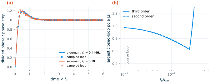
Figure 12.7a compares the response to a phase step of the reference. At the course loop’s \(f_u\) = 400 kHz, a hundredth of \(f_{ref}\), the sampled loop and the continuous-time model have the same overshoot, 18.7 %, and after allowing for the half period by which the pulses lead the averaged current they agree within 0.0714 % of the step. Scale the same filter design to \(f_u = f_{ref}/8\) = 5 MHz and the continuous-time response, plotted against \(t\,f_u\), does not change, but the sampled loop does: it overshoots by 21.7 % and departs from the model by up to 10.1 % of the step.
The poles tell the rest (Figure 12.7b). As \(f_u/f_{ref}\) rises, the largest closed-loop pole first moves inwards (the loop gets faster), then turns and leaves the unit circle at \(f_u\) = 0.294 \(f_{ref}\) for the third-order loop and 0.275 \(f_{ref}\) for the second-order loop, about \(f_{ref}/3.4\) and \(f_{ref}/3.6\). The continuous-time model, which has no notion of \(f_{ref}\), predicts a stable loop at any bandwidth. This is Gardner’s limit [135]. The usual rule, \(f_u \le f_{ref}/10\), keeps the departure from the linear model to a few per cent; the course loop, at \(f_{ref}/100\), is far inside it, and the linear noise analysis of Sections 12.3–12.4 stands.
12.7 The course synthesizer’s phase-noise budget
Choosing the charge-pump current
\(I_{CP}\) is the last free choice. At a fixed bandwidth, \(R_1 \propto 1/I_{CP}\) and \(C_{tot} \propto I_{CP}\) (Eqs. 12.4–12.5). A larger current lowers the charge pump’s in-band noise (Eq. 12.7: the signal power grows as \(I_{CP}^2\), the noise power only as \(I_{CP}\) when the devices are scaled at constant current density) and the resistors’ noise, but costs capacitor area. The script repeats the design at the chosen 400 kHz, scaling the simulated charge pump’s noise with its current:
Table 12.1. Charge-pump current against noise and area for the course loop (fu = 400 kHz, PM = 60°, third-order filter, KVCO = 131 MHz/V, simulated VCO; LO-referred).
| ICP | R1 | Ctot | L at 1 MHz | Jitter, 10 kHz–10 MHz |
|---|---|---|---|---|
| 25 µA | 98.2 kΩ | 15.9 pF | −108.6 dBc/Hz | 720 fs |
| 50 µA | 49.1 kΩ | 31.8 pF | −111.0 dBc/Hz | 555 fs |
| 100 µA | 24.5 kΩ | 63.5 pF | −113.0 dBc/Hz | 451 fs |
| 200 µA | 12.3 kΩ | 127 pF | −114.5 dBc/Hz | 388 fs |
| 400 µA | 6.13 kΩ | 254 pF | −115.5 dBc/Hz | 353 fs |
Below 50 µA the specification fails; above 100 µA each doubling of the capacitor area buys 1.5 dB or less at 1 MHz, because the reference, which no charge-pump current can improve, takes over. We take 100 µA.
The budget
Figure 12.8 is the result at the LO with the simulated VCO, and Table 12.2 breaks it down. The course synthesizer reaches −113.0 dBc/Hz at 1 MHz, 3.0 dB inside the specification, and −127.1 dBc/Hz at 3 MHz, 7.2 dB inside the −119.9 dBc/Hz that Chapter 5’s 3 MHz blocker case needs. Its rms jitter from 10 kHz to 10 MHz is 451 fs, an rms phase error of 0.396° at the LO, well below the 1.11° Chapter 5 computed for its LO mask over a similar band.
Two comparisons in Figure 12.8 say what the loop does. The free-running VCO alone, divided by two, would give −122.7 dBc/Hz at 1 MHz; inside the loop its contribution is −120.9 dBc/Hz, 1.8 dB worse, because \(1/(1+G)\) peaks near \(f_u\). The VCO was given most of the budget in Chapter 11, but the loop’s own noise takes most of the room that the VCO left. And the crystal multiplied by \(N/2\) without any loop would sit at −111.3 dBc/Hz from 100 kHz outwards: the loop keeps that only up to \(f_u\) and then hands over to the quieter VCO.
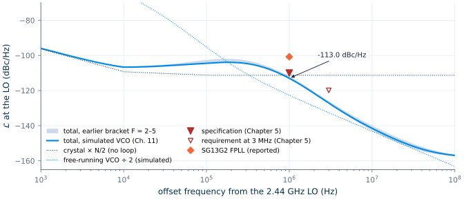
Table 12.2. Phase-noise budget of the course synthesizer at the 2.44 GHz LO (integer-N; fu = 400 kHz, ICP = 100 µA, KVCO = 131 MHz/V). Each row is one source's contribution through the closed loop; jitter integrated from 10 kHz to 10 MHz. Chapter 14 adds the ΔΣ row.
| Source (model) | 100 kHz | 1 MHz | 10 MHz | Jitter |
|---|---|---|---|---|
| TCXO, 40 MHz (datasheet, floor −147 dBc/Hz) | −110.1 | −118.8 | −157.0 | 236 fs |
| Charge pump (ngspice, 0.5 ns per period) | −110.5 | −119.2 | −157.4 | 223 fs |
| R1 = 24.5 kΩ | −115.2 | −120.6 | −158.7 | 171 fs |
| R3 = 19.0 kΩ | −116.0 | −120.9 | −148.3 | 162 fs |
| Divider, retimed (57.3 fs per edge, assumed) | −136.0 | −144.6 | −182.8 | 11.9 fs |
| Divide-by-two floor (Chapter 13) | −158.1 | −158.1 | −158.1 | 3.63 fs |
| VCO (Chapter 11, simulated: every noise source, 1/f³ corner 254 kHz) | −109.4 | −120.9 | −143.1 | 206 fs |
| ΔΣ quantization noise | Chapter 14 | |||
| Total | −104.5 | −113.0 | −141.5 | 451 fs |
| Specification (Chapter 5) | −110 |
Phase noise in dBc/Hz. The jitter of the total is the root-sum-square of the rows.
How much did the VCO simulation change? With Chapter 11’s earlier estimate in its place, a noise factor of 2–5 with an assumed 1/f³ corner of 1 MHz, the VCO row would read −109.1 to −105.1 dBc/Hz at 100 kHz and −120.6 to −116.6 dBc/Hz at 1 MHz, and the total −112.9 to −112.0 dBc/Hz at 1 MHz with 460–537 fs of jitter (the shaded band of Figure 12.8). The simulated VCO lands at the optimistic end at 1 MHz, because its 1/f³ corner, 254 kHz, is four times lower than assumed, and between the two ends above a few megahertz, where only its F = 3.71 counts. A 1 dB range has become one number; the budget’s conclusions do not change.
What this means for your design
The VCO of Chapter 11 met its specification by 12.7 dB on its own, yet the closed loop has only 3.0 dB left at 1 MHz. The margin went to the reference floor (−147 dBc/Hz × N²), to the charge pump, to two resistors, and to the loop’s own peaking. Budget the synthesizer as a whole, not the VCO alone, and give the in-band sources as much attention as the oscillator. The cheapest improvements here are a crystal with a lower floor, a shorter charge-pump on-time and a larger ICP if area allows. Chapter 14’s fractional divider will need a share of the remaining 3 dB, which is why its noise shaping and the third pole matter.
Try the loop. Move KVCO across the 103–167 MHz/V that the loop sees after band calibration, and switch between the filter designed for 131 MHz/V and the earlier one for 96.9 MHz/V. The demo forms the loop from Chapter 12’s own model (the filters’ transimpedance, every noise source of Table 12.2) and redraws the loop gain and the budget at the LO.
What the estimate leaves out
The numbers above rest on stated assumptions: the TCXO’s typical (not worst-case) phase noise, flat beyond 100 kHz; the VCO’s simulated phase noise at one operating point (code 8, Vtune = 0.6 V, typical corner, quasi-static device noise; Chapter 11 lists what that simulation leaves out); its mean KVCO at the same code; a 0.5 ns charge-pump on-time; 57.3 fs of retimed divider jitter; and noiseless buffers, bias circuits and supplies. The charge pump’s noise comes from a small-signal analysis with the sources held on, scaled by Eq. (12.10). Each could move the result by a few decibels, and the margin is 3.0 dB. Chapter 11’s simulation has already turned the VCO’s 1 dB range into one number; the next verification steps for a real design would be the VCO at the other codes and corners, the noise of the supply and of the tuning line, and a measurement-grade crystal model.
A taped-out comparison
The open-source SG13G2 fractional-N PLL of Thiriloganathan et al. [106, 207] makes an instructive comparison. It uses a 10 MHz reference, so its 2.4 GHz output is about 240 times the reference, 11.9 dB more in-band multiplication than the course synthesizer’s LO (N/2 = 61 from 40 MHz), and a third-order passive filter like ours, with two resistors of about 14.84 kΩ (rppd) and cap_cmim capacitors. Its authors report a reference spur of about −40.2 dBc and −100.8 dBc/Hz at 1 MHz. Their spur is 71.8 dB above what Eqs. (12.13)–(12.14) predict for our loop with 1 nA of leakage and 4 % mismatch (−112 dBc at the LO), which says nothing against either design: the paper’s number includes everything Section 12.5 left out (coupling, charge injection, the fractional divider), and a 10 MHz reference puts its spurs where the loop filter attenuates far less. The lesson is the same as in Chapter 11: a pre-layout estimate is a lower bound, and the distance to a measured part is made of the effects that the estimate does not model.
Try it · The PLL noise script
Every number in this chapter comes from
tools/figs/ch12_pll_noise.py:python3 tools/figs/ch12_pll_noise.pyredraws everything (the charge-pump simulation takes a second;--resimreruns it). Three experiments: (1) setXO_L[-1]to −160 dBc/Hz, the floor of a good crystal oscillator, and rerunopt budget: how far does the optimum bandwidth move, and how much margin do you gain at 1 MHz? (2) SetT_RSTto 2 ns, a long on-time like that of a fractional-N loop, and rerunnoise opt: which source now dominates in band? (3) SetRT3to 0.3 and rerunloop: does the design still have a passive solution withC3_OVER_CTOT= 0.019, and what happens to R3 if you halveC3_OVER_CTOT?
- A third-order filter adds a pole that attenuates the reference ripple (9.8 dB at 40 MHz for the course loop) without losing phase margin, if the zero and the first pole are re-centred around fu; its resistor R3 is a noise source that the design must keep small.
- Reference, divider and charge-pump noise reach the output low-passed and multiplied by N; the loop-filter resistors band-passed; the VCO high-passed. The course loop’s in-band floor is set by the crystal (−147 dBc/Hz + 20 log N) and the charge pump together.
- The integrated jitter is lowest near the bandwidth where in-band and VCO noise meet: 350 kHz for the course synthesizer with its simulated VCO; we chose 400 kHz, 2 fs from the optimum, which also keeps the 1 MHz specification and sits at fref/100. The filter is designed for the KVCO the loop sees after band calibration (131 MHz/V, the centre of 103–167 MHz/V), not for the VCO’s average or its small-signal estimate.
- Leakage and UP/DN mismatch, through Eqs. (12.12)–(12.14), give reference spurs below −100 dBc at the course loop’s values; practical spurs come from coupling and charge injection, and the third pole attenuates those too.
- The z-domain model shows the loop unstable above fu ≈ fref/3.4, which the continuous-time model cannot predict; at fref/100 the two agree within 0.1 %.
- With the VCO that Chapter 11 simulated, the course synthesizer is estimated at −113.0 dBc/Hz at 1 MHz from the LO and 451 fs of jitter, with 3.0 dB of margin for Chapter 14’s quantization noise; Chapter 11’s earlier noise-factor bracket would have given −112.0 to −112.9 dBc/Hz.
Further reading
- B. Razavi, Design of CMOS Phase-Locked Loops [11]: higher-order filters, the noise of each block, charge-pump non-idealities and spurs, at the depth of this chapter and beyond; F. M. Gardner, Phaselock Techniques [12] for the classical loop theory.
- A. L. Lacaita, S. Levantino and C. Samori, Integrated Frequency Synthesizers for Wireless Systems [21]: noise transfer functions, optimum bandwidth and the design of radio synthesizers, with fractional-N in view.
- F. M. Gardner, “Charge-pump phase-lock loops” [135], and P. K. Hanumolu et al. [136] for the sampled-loop analysis and when the continuous-time model is accurate.
- D. Banerjee, PLL Performance, Simulation, and Design [22]: closed-form designs of second-, third- and fourth-order passive filters, and practical formulas for spurs and lock time.
- S. Palermo’s ECEN 620 notes [2]: PLL noise analysis and loop design in lecture form.