Chapter 9
Low-Noise Amplifiers
The low-noise amplifier is the first active block behind the antenna: it must look like 50 Ω, add almost no noise, give enough gain to hide the mixer, and stay linear and stable. This chapter explains why the obvious ways of matching an amplifier waste noise figure, derives the inductively degenerated stage that does not, and designs the course LNA in SG13G2 from 1.2 V, with real pads, ESD diodes, spirals and capacitors, then repeats it in SKY130 and with a SiGe HBT.
- Explain why a resistively terminated stage cannot beat 3 dB and a common-gate stage not 1 + γ/α, and compute both from a transistor’s parameters.
- Derive the input impedance and the noise factor of the inductively degenerated LNA, including the effect of Cgd and of the pad capacitance.
- Size the input transistor for noise at a fixed current, and choose between an on-chip and an off-chip gate inductor.
- Design, simulate and verify a complete LNA: S-parameters, noise figure at 290 K, IIP3 and P1dB in harmonic balance, stability, corners and temperature.
- Describe resistive-feedback and noise-cancelling wideband LNAs and when a SiGe HBT is the better input device.
Contents
9.1 What an LNA must do
Chapter 4 showed with the Friis formula, Eq. (4.11), that the first gain stage sets the noise figure of a receiver: the noise of every later stage is divided by the gain in front of it. Chapter 5 turned the course radio’s targets into a block budget. For the LNA, Table 5.3 asks for a gain of +16 dB, a noise figure (NF) of 2.5 dB, an IIP3 of −6 dBm and an input reflection S11 ≤ −10 dB across 2400–2483.5 MHz, from the 1.2 V supply. Table 9.1 lists these and the requirements that are not in the budget but that every LNA must meet [6, 7].
Table 9.1. What the course LNA must do, and why.
| Requirement | Target | Why |
|---|---|---|
| Gain | ≥ 16 dB | divides the mixer’s 12 dB NF by 40 in the Friis formula |
| Noise figure (290 K) | ≤ 2.5 dB | the LNA adds directly to the receiver NF behind the 2 dB filter |
| Input match | S11 ≤ −10 dB, 2400–2483.5 MHz | the band filter is designed for 50 Ω; a mismatch changes its response and wastes signal |
| Linearity | IIP3 ≥ −6 dBm | its share of the receiver’s −12.7 dBm (Chapter 5) |
| Stability | K > 1 and μ > 1 at all frequencies | an LNA must not oscillate for any antenna or package impedance |
| Reverse isolation | S12 as small as possible | keeps LO leakage from the mixer away from the antenna |
| Supply and power | 1.2 V, a few milliwatts | shared with the rest of the receiver |
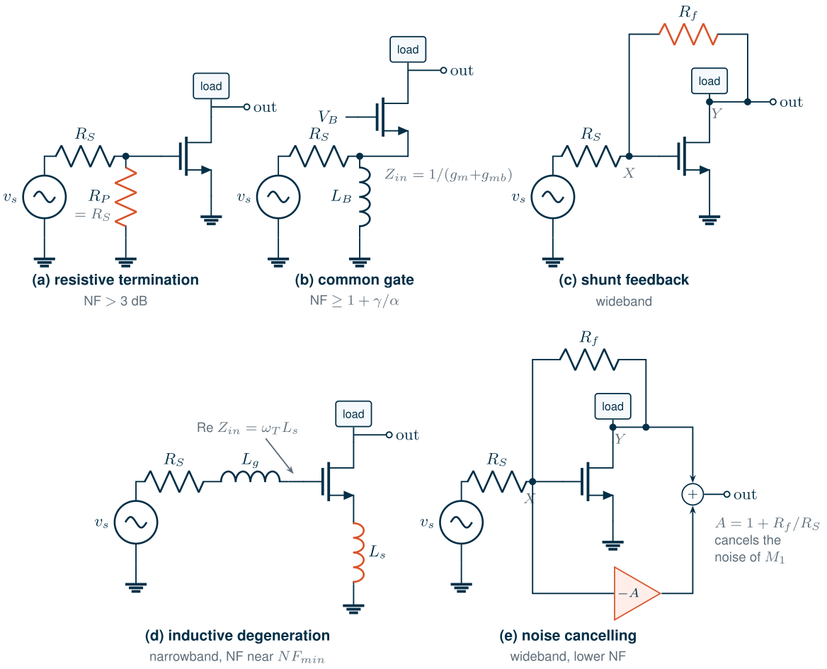
The difficulty is that the first two rows pull against the third. The noise figure of a two-port is lowest for one source impedance, Zopt (Eq. (6.11)), while the input match asks the amplifier’s input impedance to be the conjugate of the source. For a MOSFET the two are far apart: Chapter 6 found Zopt = 1160 + j2140 Ω for a 20 µm SG13G2 device at 2.4 GHz, and an input that is almost purely capacitive. An LNA topology is a way of making the input look like 50 Ω while keeping the source close to Zopt, and without adding noisy resistors on the way. Figure 9.1 shows the five ways this chapter studies.
9.2 The resistively terminated common-source stage
The simplest match is a resistor RP = RS from the gate to a bias voltage (Figure 9.1a). It works at any frequency, but it is a noisy resistor of exactly the source’s value in parallel with the input. The source sees half its own noise voltage at the gate, and the terminating resistor adds as much again. Chapter 4 derived the noise factor, Eq. (4.9), which we repeat because it is the baseline of this chapter:
Key equation · Noise factor of a resistively terminated stage
\[F = 2 + \frac{4R_n}{R_S} + \frac{4}{g_m^2 R_D R_S} \;\geq\; 2. \tag{9.1}\]\(R_n = R_g + \gamma/g_m\) is the transistor’s noise resistance and \(R_D\) its load. Even a noiseless transistor leaves F = 2, an NF of 3 dB.
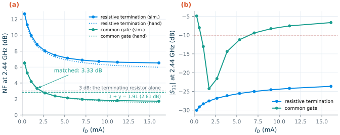
The topo part of the chapter script simulates the stage with the course device, 8 cells of 4 × 2/0.13 µm (64 µm, Rg = 6.72 Ω in the RF model) and a 2 kΩ load, and sweeps the gate bias (Figure 9.2). The match is excellent (S11 ≤ −23.7 dB everywhere), but the NF falls only to 6.52 dB at 16.1 mA. Eq. (9.1) with Chapter 4’s γ = 0.91 follows the simulation; the transistor’s Rn keeps the NF far above even the 3 dB floor. A resistively terminated LNA is acceptable only where noise does not matter, for example as a test buffer.
9.3 The common-gate LNA
Drive the source of a MOSFET instead of its gate (Figure 9.1b). The source current returns through the channel, so the input looks like a conductance gm, plus gmb because the source also moves against the bulk:
\[Z_{in} \approx \frac{1}{g_m + g_{mb}}. \tag{9.2}\]A bias current of a couple of milliamperes gives 50 Ω over a wide band, with no noisy resistor. The noise, however, is now set by gm itself. The channel noise current \(4kT\gamma g_m\) splits between the channel and the source resistance, and only the part that stays in the channel reaches the drain. With \(g_i = g_m + g_{mb}\) and \(\chi = g_{mb}/g_m\) [6]:
Key equation · Noise factor of the common-gate stage
\[F = 1 + \frac{\gamma g_m}{g_i^2 R_S} + \frac{R_g g_m^2}{g_i^2 R_S} + \frac{(1 + g_iR_S)^2}{g_i^2 R_S R_D}, \tag{9.3}\] \[F\big\vert_{g_iR_S = 1} = 1 + \frac{\gamma}{1 + \chi} + \frac{R_g}{R_S(1+\chi)^2} + \frac{4R_S}{R_D}. \tag{9.4}\]At match the channel term is \(\gamma/(1+\chi)\) whatever the current. With γ referred to the zero-bias channel conductance \(g_{d0}\), as in long-channel theory, it reads \(\gamma/\alpha\) with \(\alpha = g_m/g_{d0}\): the classic bound F ≥ 1 + γ/α.
Derivation · Noise factor of the common-gate stage
Short the input source to its resistance RS and ignore ro. A signal voltage vs drives a current \(v_s g_i/(1 + g_iR_S)\) into the source, and all of it flows to the drain. The channel noise current \(i_n\) (density \(4kT\gamma g_m\)) flows from drain to source inside the device; at the source node it sees RS in parallel with \(1/g_i\), so a fraction \(1/(1 + g_iR_S)\) of it circulates through the drain. A gate-resistance noise voltage \(v_g\) (\(4kTR_g\)) acts like a gate signal and gives a drain current \(g_mv_g/(1 + g_iR_S)\). The load’s noise current \(4kT/R_D\) adds directly at the drain. Dividing each output noise power by the output noise due to RS, \(4kTR_S\,g_i^2/(1 + g_iR_S)^2\), gives the four terms of Eq. (9.3).
Figure 9.2 shows the trade. The common-gate stage is matched (S11 = −24.3 dB) at 1.75 mA, where gm = 15.9 mS: gmRS is only 0.796 because gmbRS = 0.091 helps, and the drain conductance does the rest. There the NF is 3.33 dB, and Eq. (9.3) gives 3.31 dB. The floor 1 + γ is 2.81 dB, or 2.59 dB with the body effect’s χ = 0.114. More current lowers the NF (1.73 dB at 16.1 mA) only by spoiling the match. The common gate is therefore a wideband LNA with a mediocre noise figure, and a building block of noise-cancelling and balun LNAs (Section 9.6).
9.4 The inductively degenerated common-source LNA
Input impedance
The input of a common-source MOSFET is a capacitor, which has no real part to match. An inductor Ls in the source creates one (Figure 9.1d) [110, 7]. A gate current i charges Cgs to \(v_{gs} = i/(j\omega C_{gs})\), and the drain current \(g_mv_{gs}\) flows through Ls and develops \(j\omega L_s\,g_m\,i/(j\omega C_{gs}) = (g_m L_s/C_{gs})\,i\), in phase with i. The source inductance turns the transconductance into a resistance that is not a resistor and adds no thermal noise. With a gate inductor Lg in series:
\[Z_{in} = j\omega(L_g + L_s) + \frac{1}{j\omega C_{gs}} + R_g + \frac{g_m}{C_{gs}}L_s. \tag{9.5}\]Key equation · Input of the inductively degenerated stage
\[\mathrm{Re}\,Z_{in} = R_g + \omega_T L_s, \quad \omega_T = \frac{g_m}{C_{gs}}, \qquad \omega_0 = \frac{1}{\sqrt{(L_g + L_s)\,C_{gs}}}. \tag{9.6}\]Ls sets the real part, Lg resonates Cgs at the band centre ω0. The match is narrowband by nature.
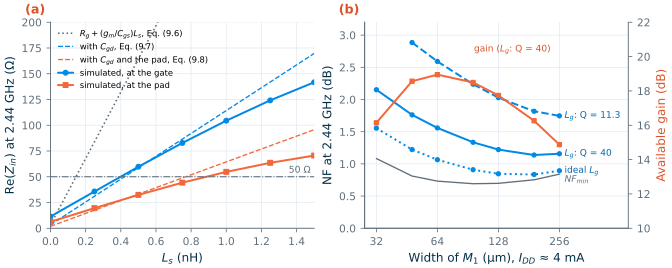
In SG13G2 the textbook formula is far off. The course input device, 128 µm at its LNA bias (VGS = 0.664 V), has gm = 38.6 mS, Cgs = 120 fF and Cgd = 67.8 fF: Cgd is 36 % of Cgg in this short-channel RF model. Eq. (9.6) predicts a slope of gm/Cgs = 322 Ω/nH, but the simulated Re(Zin) at the gate rises only 93.1 Ω per nH (Figure 9.3a). Part of the gate current flows through Cgd into the cascode node, which swings with a gain of about one, and never passes through Ls. Including that path (derivation below):
\[\mathrm{Re}\,Z_{in} \approx R_g + \omega_T L_s\left(\frac{C_{gg}}{C_{gg} + C_{gd}}\right)^2, \qquad \omega_T = \frac{g_m}{C_{gg}}, \tag{9.7}\]which gives 111 Ω/nH, within 20 % of the simulation. The bond pad and the ESD diodes add a capacitance Cpad from the gate node to ground, 84.7 fF here (Section 9.7). It takes its share of the current as well:
\[\mathrm{Re}\,Z_{in,pad} \approx \mathrm{Re}\,Z_{in}\left(\frac{C_{gg} + C_{gd}}{C_{gg} + C_{gd} + C_{pad}}\right)^2. \tag{9.8}\]The pad halves the slope (62.5 Ω/nH predicted, 48.4 Ω/nH simulated). For 50 Ω the textbook formula asks for Ls = 0.145 nH, Eq. (9.7) for 0.421 nH and Eq. (9.8) for 0.769 nH; the simulation needs 0.887 nH (ideal Ls, at the pad). The hand formulas show the trends; the value comes from the simulator.
Derivation · The input resistance with Cgd
Let the cascode node x follow \(v_x \approx -(g_m/g_{m2})v_{gs} \approx -v_{gs}\), and neglect the current of Cgs in Ls against \(g_mv_{gs}\). The gate current is \(i = j\omega C_{gs}v_{gs} + j\omega C_{gd}(v_g - v_x) \approx j\omega(C_{gs} + 2C_{gd})v_{gs}\), so the fraction of the gate current that flows into Cgs is \(C_{gs}/(C_{gs} + 2C_{gd})\). Only that fraction makes drain current, so the voltage across Ls is \(j\omega L_s g_m v_{gs} = g_mL_s\,i/[j\omega(C_{gs} + 2C_{gd})]\), and dividing by the current into the input capacitance \(j\omega(C_{gs} + 2C_{gd})\) once more gives \(\mathrm{Re}\,Z_{in} = g_mL_s(C_{gs} + C_{gd})/(C_{gs} + 2C_{gd})^2\) to first order in \(\omega L_sg_m\). With \(C_{gs} + C_{gd} = C_{gg}\) this is Eq. (9.7). A shunt Cpad in front divides the current again in the ratio of the capacitances, which squares into Eq. (9.8).
Noise
At resonance and with the input matched, \(g_mL_s/C_{gs} = R_S\), and the loop current that the channel noise drives through Ls cancels half of it: only \(i_n/2\) reaches the drain, while the signal arrives multiplied by the input network’s voltage gain. The result is remarkably simple [6, 110]:
Key equation · Noise factor of the inductively degenerated LNA
\[F = 1 + \frac{R_{Lg} + R_g + R_{Ls}}{R_S} + \gamma\,g_m R_S\left(\frac{\omega_0}{\omega_T}\right)^2, \tag{9.9}\] \[Q_L = \frac{\omega_0(L_g + L_s)}{R_S} = \frac{1}{\omega_0 R_S C_{gs}}, \qquad \gamma\,g_m R_S\left(\frac{\omega_0}{\omega_T}\right)^2 = \frac{\gamma}{Q_L}\,\frac{\omega_0}{\omega_T}. \tag{9.10}\]Every resistance in series with the source counts in full; the channel’s contribution falls with ωT/ω0. Unlike Eqs. (9.1) and (9.4) nothing forces F above a fixed floor.
Derivation · Why half the channel noise reaches the output
With vs = 0, let the channel noise current \(i_n\) flow from drain to source and let \(i_g\) be the loop current through RS, Lg and Cgs. The source node carries \(i_g + g_mv_{gs} + i_n\) into Ls, with \(v_{gs} = i_g/(j\omega C_{gs})\). Around the loop, \(i_g\left[R_S + j\omega(L_g + L_s) + 1/(j\omega C_{gs}) + g_mL_s/C_{gs}\right] = -j\omega L_s i_n\). At resonance the reactances cancel and at match \(g_mL_s/C_{gs} = R_S\), so \(i_g = -j\omega L_si_n/(2R_S)\) and the drain current is \(g_mv_{gs} + i_n = i_n\left[1 - g_mL_s/(2R_SC_{gs})\right] = i_n/2\). The signal gives \(i_g = v_s/(2R_S)\) and \(\vert i_d\vert = v_s\,\omega_T/(2\omega_0 R_S)\). The ratio of \(\overline{i_n^2}/4 = kT\gamma g_m\) to the output noise of RS, \(4kTR_S\,\omega_T^2/(4\omega_0^2R_S^2)\), is the last term of Eq. (9.9).
Eq. (9.9) leaves out one physical effect. The fluctuating channel charge also couples a noise current onto the gate through Cgs, the induced gate noise, which grows with frequency and is partly correlated with the drain noise [18, 110]. Its voltage across the input network grows with QL, while the channel term of Eq. (9.10) falls with it, so there is an optimum. Shaeffer and Lee found that at a fixed bias current, for long-channel parameters, the noise figure is lowest at QL ≈ 4.5, which fixes the width [110, 111]:
\[W_{opt} \approx \frac{1}{3\,\omega_0 L C_{ox} R_S}. \tag{9.11}\]For SG13G2 (Cox = 14.1 fF/µm², L = 0.13 µm) at 2.44 GHz this is 237 µm. The sizing sweep of Figure 9.3b, in which ngspice includes whatever gate noise the PSP model carries, finds the minimum NF with an ideal gate inductor at 192 µm (0.83 dB), where QL = 3.8. The minimum is broad: from 96 to 256 µm the NF stays within 0.1 dB of it. The gain is not: the available gain falls from 18.5 dB at 96 µm to 14.9 dB at 256 µm, because a wider device has a lower ωT. The course LNA uses 128 µm, 0.08 dB from the noise minimum with a Q = 40 gate inductor (1.22 against 1.14 dB) and 1.4 dB more gain than 192 µm. Extra capacitance in parallel with Cgs moves the optimum to smaller devices and lower currents, the idea of power-constrained simultaneous noise and input matching [112]; Section 9.8 uses it for the HBT.
The gate inductor: on chip or off chip?
Figure 9.3b also shows what matters most: the loss of Lg, which sits in series with the source and enters Eq. (9.9) in full. At 128 µm, Lg must be 13.5 nH. That is three times the largest spiral of Chapter 7’s EM-fitted family (4.94 nH), whose single-ended Q at 2.44 GHz is only 11.3. Even at that optimistic Q, an on-chip Lg would raise the NF from 1.22 to 2.03 dB; a real 13 nH spiral would be larger, lossier and closer to its self-resonance. The course LNA therefore puts Lg on the board: a 0402 wire-wound chip inductor plus the bond wire. We model it as an ideal inductance with a series resistance for Q = 40, a value typical of such parts at 2.4 GHz (an assumption, not a measured part). The source inductor (0.82 nH) and the load inductor (2.5 nH) are small enough to be the spirals of Chapter 7.
Common pitfall · An ideal gate inductor
Simulated with an ideal Lg, the course LNA has an NF of 0.75 dB; with the Q = 40 chip inductor it has 1.17 dB, and with a Q of 11.3 it would have 2.09 dB (Section 9.7). The gate inductor’s loss is the largest single noise contribution of a narrowband LNA. Never quote an LNA’s noise figure without stating the Q of Lg and whether the pad, the bond wire and the ESD protection are included.
9.5 Gain, cascodes and stability
The cascode
M1 alone would see the full drain swing across its large Cgd: the Miller effect would multiply it, couple the output back to the tuned input and make S12 large. A common-gate transistor M2 on top (the cascode) holds the drain of M1 at a low impedance node x. In the course LNA M2 has the same 16 cells as M1 and its gate at VDD, which leaves 0.498 V across M1. The reverse transmission is S12 = −38.1 dB at 2.44 GHz, and the input match no longer depends on the load.
Gain
At resonance the input network magnifies the source voltage onto Cgs, so the stage’s effective transconductance is
\[G_m = \frac{i_{out}}{v_s} = g_m\left\vert\frac{v_{gs}}{v_s}\right\vert \approx \frac{\omega_T}{2\omega_0 R_S} = \frac{g_m Q_L}{2}. \tag{9.12}\]In the harmonic-balance simulation of the course LNA, \(\vert v_{gs}\vert\) is 1.65 times the source’s open-circuit voltage, so Gm = 1.65 × 38.6 mS = 63.7 mS; the pad and Cgd make the magnification smaller than QL/2 = 2.27. The drain drives a tuned load: a 2.5 nH spiral (Q = 11.0 at 2.44 GHz) resonated by the device capacitance and by a tapped-capacitor match of a series C1 and a shunt C2, which transforms the 50 Ω load up to the conjugate of the drain’s output impedance (matching networks are the subject of Chapter 8). The resulting power gain is about \(G_m^2 R_S\) times the resistance at the drain, so the load resistance, set by Ld and its Q, decides the gain.
Gain against linearity
The same drain resistance also decides how far the drain swings. Table 9.2 repeats the design for four load inductors, with Ls, Lg and the output match redone each time. A larger Ld raises the gain by 2.9 dB from 2 to 3.5 nH, but the IIP3 falls by 4.2 dB: the output intercept OIP3 = IIP3 + G stays between +11.6 and +12.9 dBm, because the drain runs out of voltage swing between VDD and the cascode node, whatever the gain. The specification pair G ≥ 16 dB and IIP3 ≥ −6 dBm needs OIP3 ≥ +10 dBm, so the margin must be split between the two. Ld = 2.5 nH leaves 1.4 dB of gain margin and 1.1 dB of IIP3 margin.
Table 9.2. Gain against linearity: the course LNA with four load inductors (each rematched; 4.7 mA, tt, 27 °C; IIP3 from two tones at 2.440/2.441 GHz in Xyce).
| Ld | S21 at 2.44 GHz | NF | IIP3 | OIP3 |
|---|---|---|---|---|
| 2.0 nH | 16.4 dB | 1.19 dB | −3.5 dBm | +12.9 dBm |
| 2.5 nH (design) | 17.61 dB | 1.17 dB | −4.9 dBm | +12.7 dBm |
| 3.0 nH | 18.53 dB | 1.16 dB | −6.3 dBm | +12.2 dBm |
| 3.5 nH | 19.27 dB | 1.15 dB | −7.7 dBm | +11.6 dBm |
Stability
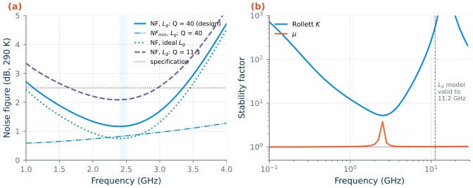
An LNA faces an unknown antenna and package, so it must be unconditionally stable, \(K > 1\) and \(\vert\Delta\vert < 1\), or \(\mu > 1\) (Eq. (3.24)), at every frequency where it has gain, not only in the band. The course LNA’s K is at least 5.23 (at 2.51 GHz) and μ at least 1.02 above 1 GHz (Figure 9.7b). Below 1 GHz μ approaches 1.000 from above: the DC blocks make both ports nearly lossless reflections there, and \(\mu \to 1/\vert S_{22}\vert\), which is just above one. The cascode, the losses of the spirals and the source degeneration keep the amplifier far from oscillation; the gain at 10 GHz is −43.4 dB. Above 11.2 GHz the curves are only indicative, because the EM-fitted model of Ld is not valid there; a stability check of the real layout needs its extracted parasitics (Chapter 18).
9.6 Wideband and noise-cancelling LNAs
A narrowband LNA serves one band. A receiver that covers several bands, or a software-defined radio, needs an input that is matched over octaves, which neither Eq. (9.6) nor any resonant network gives. Two wideband ideas are shown here with short simulations (part wide).
Resistive shunt feedback
A resistor Rf from the output of an inverting amplifier back to its input (Figure 9.1c) lowers the input resistance by the loop gain:
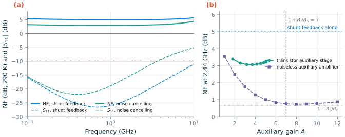
\[R_{in} \approx \frac{R_f + R_L}{1 + g_m R_L}. \tag{9.13}\]The amplifier is a CMOS inverter (8 n-cells and 16 p-cells of 4 × 2/0.13 µm, rfmode=1), which self-biases at 0.611 V through Rf = 300 Ω and reuses its current in both devices. It draws 1.51 mA (1.81 mW) and is matched (S11 ≤ −10 dB) from 0.1 to 10 GHz, with 7.92 dB of gain at 1 GHz and 5.29 dB at 5 GHz (Figure 9.4a). Its NF is 5.03 dB at 2.44 GHz: Rf and the transistors’ noise appear at the input almost undivided. Port 2 is driven through an ideal buffer with a noiseless 50 Ω output resistance, so that the numbers describe the LNA core.
Noise cancelling
Bruccoleri, Klumperink and Nauta observed that the main transistor’s noise current flows out through Rf and RS, so it produces voltages of the same sign at the input X and the output Y, in the ratio \(1 + R_f/R_S\); the signal appears with opposite signs [113]. An auxiliary amplifier of gain −A that senses X and is added to Y (Figure 9.1e) therefore cancels the noise and adds the signal when
\[A = 1 + \frac{R_f}{R_S}, \qquad F \rightarrow 1 + \frac{R_S}{R_f} + F_{aux} - 1. \tag{9.14}\]The match is still set by Rf, which is the point: noise and match are decoupled. Figure 9.4b tests Eq. (9.14). With a noiseless auxiliary amplifier the NF falls to 0.76 dB at A = 7, and its minimum, 0.74 dB at A = 8, sits on the floor 1 + RS/Rf (0.67 dB): Rf’s own noise is not cancelled. With a real auxiliary stage, a common-source nMOS of 16 cells with Ra = 150 Ω, the best NF is 3.06 dB at A = 3.71. The auxiliary transistor’s own noise moves the optimum below the cancellation point, and at 1.2 V its load cannot reach A = 7 without pushing it into triode. The complete noise-cancelling LNA draws 4.71 mA (5.65 mW), has 11.82 dB of gain and is matched from 0.1 to 3.55 GHz; the auxiliary device’s gate capacitance limits the band. The balun-LNA of Blaakmeer et al. applies the same idea to a common-gate input and a common-source auxiliary path [114].
What this means for your design
At the same 5.6 mW, the noise-cancelling LNA reaches 3.06 dB over 0.1–3.55 GHz and the inductively degenerated LNA 1.17 dB over one band. The course radio has one band and a band filter in front, so it uses the narrowband LNA. Choose a wideband LNA when the band, not the noise figure, is the hard requirement.
9.7 The course LNA at 2.4 GHz
The circuit
Figure 9.5 shows the complete design. Every element is a model that exists in the process or on the board:
- Input device: M1, 16 RF cells of 4 fingers × 2/0.13 µm (128 µm), so the model’s 40 Ω per cell becomes Rg = 3.36 Ω (Eq. (6.6)). It carries 4.39 mA, 0.0343 mA/µm; the whole LNA draws 4.70 mA, 5.64 mW from 1.2 V.
- Bias: one cell MB in a 1:16 mirror fed with 0.313 mA, through RB = 20 kΩ; CB filters the mirror’s noise. A mirror tracks process and temperature, which the corner check below relies on.
- Pad and ESD: an 80 µm pad (30 fF, estimated as a parallel plate with fringing over a Metal1 shield) and SG13G2’s 2 kV ESD diodes to VDD and ground, which add 54.7 fF at their bias: 84.7 fF in total. Chapter 18 later found 37.2 fF for the pad by EM; with it the worst in-band S11 rises from −15.4 to −13.5 dB, still within specification, and gain and noise figure barely move.
- DC block: a 2.4 pF cap_rfcmim (39.9 µm square, 10 µm feed) between pad and gate.
- Inductors: Lg = 14.0 nH off chip (Q = 40); Ls = 0.823 nH and Ld = 2.5 nH from the EM-fitted spirals of Chapter 7, with Q = 9.41 and 11.0 at 2.44 GHz.
- Output match: C1 = 2.44 pF and C2 = 3.89 pF, cap_rfcmim.
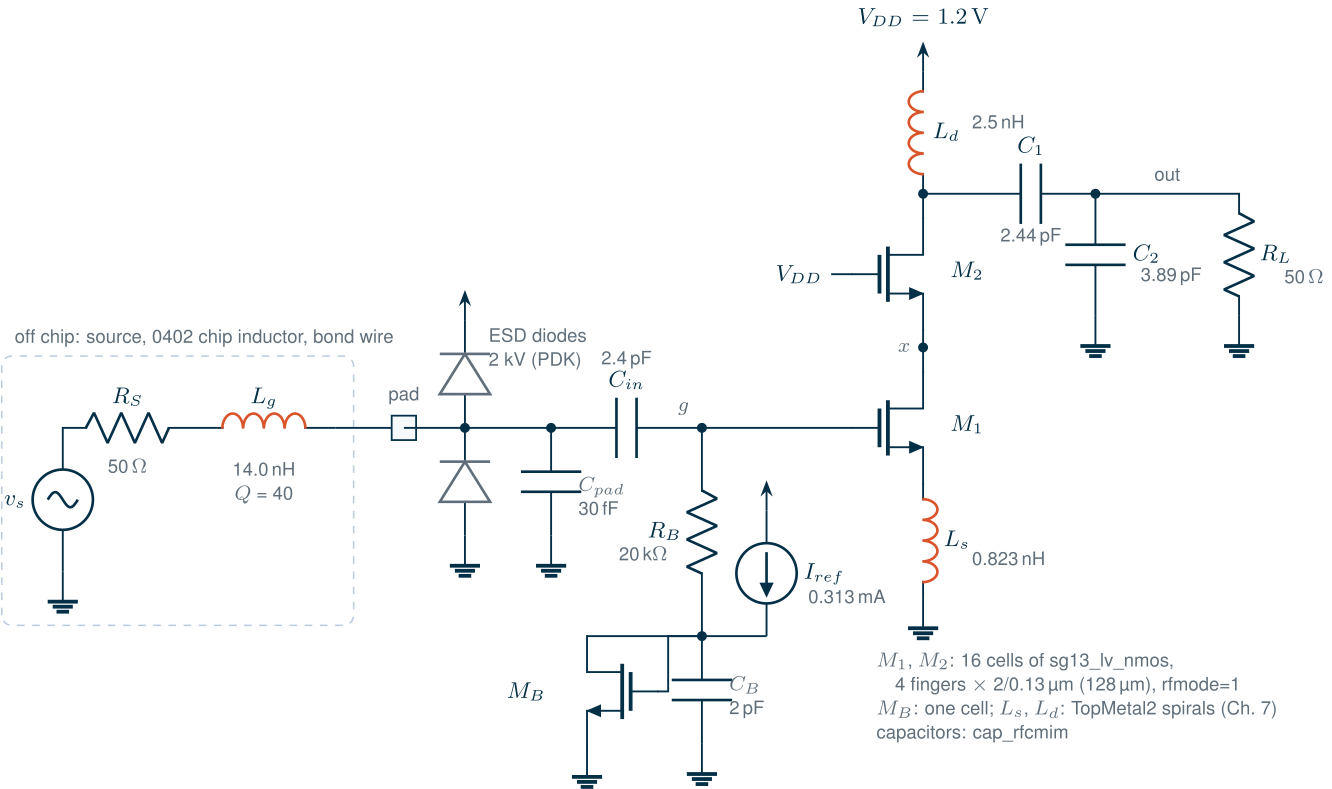
The design follows the steps of Section 9.4, done by the design part of the script: simulate the core (port 1 at the pad, port 2 at the drain) for three spirals, interpolate Ls for Re(Zin) + RLg = 50 Ω, choose Lg for resonance, compute C1 and C2 in closed form for a conjugate output match, then scale C1 and C2 (by 0.96) for the flattest gain, because cap_rfcmim’s parasitics add capacitance at the drain. The core alone has an available gain of 18.59 dB and an NF of 1.15 dB.
* course LNA, SG13G2 (ports for ngspice's sp analysis; .lib cornerCAP.lib cap_typ, cornerDIO.lib dio_tt)
v1  p1 0 dc 0 ac 1 portnum 1 z0 50
Lg  p1 lg1 14.0n                       ; off chip, Q = 40:
Rlg lg1 pad 5.36
Cpad pad 0 30f
XD1 vdd pad 0 diodevdd_2kv             ; 2 kV ESD diodes
XD2 vdd pad 0 diodevss_2kv
XCin pad g 0 cap_rfcmim w=39.95u l=39.95u wfeed=10u
iref vdd nb 312.5u
XMB nb nb 0 0 sg13_lv_nmos W=8u L=0.13u ng=4 m=1 rfmode=1
XCB nb 0 0 cap_rfcmim w=36.46u l=36.46u wfeed=10u
RB  nb g 20k
XM1 x g s 0 sg13_lv_nmos W=8u L=0.13u ng=4 m=16 rfmode=1
XM2 d vdd x 0 sg13_lv_nmos W=8u L=0.13u ng=4 m=16 rfmode=1
* Ls (0.823 nH, s to 0) and Ld (2.5 nH, vdd to d): inductor_lines() of tools/figs/_ch07_inductor.py
XC1 d out 0 cap_rfcmim w=40.25u l=40.25u wfeed=10u
XC2 out 0 0 cap_rfcmim w=50.89u l=50.89u wfeed=10u
v2  out 0 dc 0 ac 1 portnum 2 z0 50
.control
op
sp lin 301 1e9 4e9 1                   ; NF referred to 27 C: convert to 290 K
.endc
* the same LNA with SKY130 nfet_01v8 (VDD = 1.2 V); passives identical or ideal
* the model has no gate resistance: the layout estimate of Eq. (6.5), 32.4 ohm per cell, divided by 16
RM1g g g_M1 2.02
XM1 x g_M1 s 0 sky130_fd_pr__nfet_01v8 W=8 L=0.15 nf=4 mult=16 m=16 ad=... as=... pd=... ps=...
RM2g vdd vdd_M2 2.02
XM2 d vdd_M2 x 0 sky130_fd_pr__nfet_01v8 W=8 L=0.15 nf=4 mult=16 m=16 ad=... as=... pd=... ps=...
Cpad pad 0 84.7f                       ; pad + the SG13G2 ESD capacitance, as a linear capacitor
* rematched: Ls = 0.849 nH, Lg = 17.3 nH, C1 = 2.57 pF, C2 = 4.24 pF (ideal capacitors)
Small-signal results
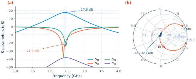
Figure 9.6 shows the S-parameters. The gain is 17.61 dB at 2.44 GHz and at least 17.43 dB across the band. S11 is −20.97 dB at the centre and no worse than −15.39 dB in the band; it stays below −10 dB from 2.23 to 2.61 GHz, a 379 MHz return-loss bandwidth set by QL = 4.54. S22 is −19.48 dB at the centre. On the Smith chart S11 passes close to the centre across the band.
The noise figure, referred to 290 K as in Chapter 4, is 1.17 dB at 2.44 GHz and at most 1.18 dB in the band; NFmin is 0.83 dB (Figure 9.7a). With an ideal gate inductor the NF would be 0.75 dB, and with an on-chip-like Q of 11.3, 2.09 dB.
Worked example 9.1 · The noise budget of the course LNA
Eq. (9.9), term by term. The chip inductor has \(R_{Lg} = \omega_0L_g/Q\) = 5.36 Ω, which adds 0.107 to F; the gate resistance Rg = 3.36 Ω adds 0.0672; the source spiral’s 1.34 Ω adds 0.0268. For the channel term, use the effective ωT of the stage that the input actually sees, the slope of Re(Zin) at the pad, 48.4 Ω/nH, that is \(\omega_T\) = 2π × 7.7 GHz: with γ = 0.91 and gm = 38.6 mS it adds 0.176. In total F = 1.38, an NF of 1.39 dB, against 1.17 dB (F − 1 = 0.309) simulated. The hand estimate is 0.2 dB pessimistic, mostly in the channel term, but it gets the ranking right: the gate inductor, the channel and the gate resistance, in that order, and the losses in series with the source together make more than half of the excess noise.
Linearity from harmonic balance
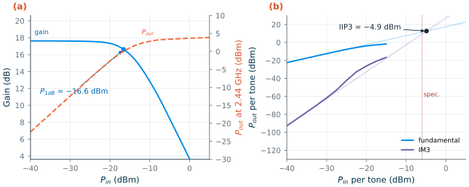
Xyce’s harmonic balance gives the large-signal behaviour (Figure 9.8). Its small-signal gain at −40 dBm is 17.62 dB, 0.01 dB from ngspice’s S21, which confirms that both simulators see the same circuit (see the PDK note). The input-referred 1 dB compression point is −16.6 dBm (output 0.0 dBm). Two tones at 2.440 and 2.441 GHz give IIP3 = −4.9 dBm (OIP3 = +12.7 dBm), extrapolated from the three lowest drive levels, where the fundamental and IM3 rise with slopes of 1.00 and 3.04. Between −27.5 and −20 dBm the IM3 rises faster, with a slope of 3.57, as fifth-order terms take over, and above −15 dBm per tone the harmonic balance no longer converges; the intercept is therefore taken where the third-order law holds. The gap of 11.7 dB between IIP3 and P1dB is close to the 9.6 dB of a memoryless third-order nonlinearity (Eq. (4.18)).
SG13G2 · Xyce does apply rfmode=1
Earlier chapters assumed that Xyce ignores SG13G2’s
rfmodeswitch. In the IIC-OSIC-TOOLS 2026.10 Xyce models the RF parameters are expressions ofrfmodeinside the single PSP model card, sorfmode=1on the instance switches on the gate resistance, the substrate network and the extra gate capacitance; only the non-quasi-static channel (swnqs) is missing, because Xyce loads the plain PSP 103 plugin. A Xyce AC analysis of Chapter 6’s reference device gives an input resistance at 10 GHz of 5.01 Ω withrfmode=0and 25.7 Ω withrfmode=1, against 25.5 Ω from Eq. (6.6). The harmonic-balance netlists of this chapter therefore userfmode=1and do not add the gate resistance by hand, which would count it twice.
Corners and temperature
Table 9.3 repeats the band sweep and the two-tone test at the slow and fast MOSFET corners and at −40 and 85 °C (passives typical, the reference current constant). The mirror holds the current between 4.47 and 5.01 mA, and the LNA meets every specification at every point: gain at least 17.06 dB, NF at most 1.40 dB (at 85 °C, where every resistor is noisier), S11 at most −13.7 dB and IIP3 between −5.7 and −4.5 dBm.
Table 9.3. The course LNA at the MOSFET corners and at three temperatures (2.40–2.49 GHz; NF referred to 290 K; IIP3 at 2.44 GHz from Xyce).
| Corner, temperature | IDD | S21 min–max | NF max | S11 max | IIP3 |
|---|---|---|---|---|---|
| tt, −40 °C | 4.61 mA | 17.67–17.83 dB | 0.93 dB | −15.5 dB | −4.5 dBm |
| tt, 27 °C | 4.70 mA | 17.43–17.61 dB | 1.18 dB | −15.4 dB | −4.9 dBm |
| tt, 85 °C | 4.80 mA | 17.06–17.28 dB | 1.39 dB | −15.0 dB | −5.1 dBm |
| ss, −40 °C | 4.47 mA | 17.74–17.89 dB | 0.93 dB | −17.4 dB | −4.5 dBm |
| ss, 27 °C | 4.54 mA | 17.48–17.63 dB | 1.18 dB | −17.1 dB | −4.9 dBm |
| ss, 85 °C | 4.61 mA | 17.08–17.25 dB | 1.40 dB | −16.5 dB | −5.0 dBm |
| ff, −40 °C | 4.79 mA | 17.68–17.88 dB | 0.93 dB | −14.1 dB | −4.7 dBm |
| ff, 27 °C | 4.91 mA | 17.47–17.69 dB | 1.17 dB | −14.0 dB | −5.3 dBm |
| ff, 85 °C | 5.01 mA | 17.12–17.37 dB | 1.38 dB | −13.7 dB | −5.7 dBm |
The same LNA in SKY130
Replacing the transistors by SKY130’s nfet_01v8, with the same cells, current reference and supply, and the rest identical or ideal (the SG13G2 spirals, ideal capacitors, the 84.7 fF of pad and ESD as a linear capacitor), and rematching gives Ls = 0.849 nH and Lg = 17.3 nH. The SKY130 LNA draws 3.66 mA (4.40 mW); its higher threshold puts the gate at 0.894 V and leaves only 0.305 V across M1. It reaches 18.53 dB of gain and an NF of 1.20 dB, practically the course LNA’s numbers at 22 % less power (Figure 9.9). The reason is in the device: at its bias the SKY130 transistor has Cgd = 32.4 fF, half of SG13G2’s, so less of the gate current bypasses Ls and the input network magnifies more.
SG13G2 vs SKY130 · The missing gate resistance
SKY130’s nfet_01v8 model has no gate resistance and no NQS channel, so the SKY130 LNA includes the layout estimate of Chapter 6 (Eq. (6.5)): 2.02 Ω for 16 cells. Without it the NF comes out at 1.13 dB instead of 1.20 dB, and with an ideal transistor model the comparison would flatter SKY130 further. Its stability margin is also optimistic: with so little loss in the model, μ stays above one but approaches 1.000 near 28 GHz. SG13G2’s RF model, with 40 Ω per cell, NQS and a substrate network, is the more pessimistic and the more trustworthy of the two.
9.8 SiGe HBT LNAs
A bipolar transistor gives \(g_m = I_C/V_T\), about four times the transconductance per milliampere of the course MOSFET, so an HBT LNA can reach the same gain at less current. Its noise sources differ (Chapter 6, Eq. (6.13)): shot noise of the base and collector currents and the thermal noise of rb, instead of channel and gate noise. The hbt part keeps the topology and replaces M1 by an npn13G2 with eight emitter fingers, cascoded by the same lv nMOS M2 (an HBT cascode does not fit under 1.2 V). Its ωT is so high that Ls for 50 Ω would be far below the smallest fitted spiral (0.424 nH), so a 0.3 pF MIM capacitor Cex across base and emitter lowers it, the power-constrained matching idea of Section 9.4 [112]. Then Ls = 0.636 nH and Lg = 10.0 nH.
At 1.43 mA in the HBT (1.68 mA, 2.02 mW in total) the HBT LNA has 17.12 dB of gain (16.93 dB minimum in the band), an NF of 1.29 dB and S11 ≤ −21.85 dB (Figure 9.9). It needs 36 % of the MOSFET LNA’s power for 0.5 dB less gain and 0.12 dB more noise. At 2.4 GHz the HBT’s advantage is power, not noise; at 50 GHz it is noise as well, where Chapter 6 found an NFmin of 1.33 dB for the npn13G2 against 3.55 dB for the nMOS, which is why the millimetre-wave front end of Chapter 17 is bipolar.
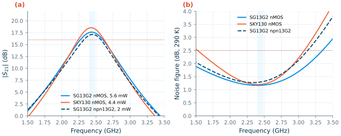
Results against the specification
Table 9.4. The course LNA against the LNA specification of Table 5.3 (SG13G2, tt, 27 °C; band 2400–2483.5 MHz, simulated 2.40–2.49 GHz), with the SKY130 and HBT versions for comparison.
| Parameter | Specification | Course LNA (SG13G2 nMOS) | Pass | SKY130 nMOS | npn13G2 |
|---|---|---|---|---|---|
| Gain S21 (band minimum) | ≥ 16 dB | 17.43 dB | ✓ | 18.23 dB | 16.93 dB |
| NF at 290 K (band maximum) | ≤ 2.5 dB | 1.18 dB | ✓ | 1.22 dB | 1.32 dB |
| S11 (band maximum) | ≤ −10 dB | −15.39 dB | ✓ | −15.83 dB | −21.85 dB |
| IIP3 (2.44 GHz) | ≥ −6 dBm | −4.9 dBm | ✓ | — | — |
| P1dB (input) | — | −16.6 dBm | — | — | |
| S22 (band maximum) | — | −12.71 dB | −14.49 dB | −11.54 dB | |
| S12 (2.44 GHz) | — | −38.12 dB | |||
| Stability | K, μ > 1 | K ≥ 5.23, μ > 1 (0.1–30 GHz) | ✓ | K ≥ 3.63 | K ≥ 25.8 |
| Supply, power | 1.2 V | 4.70 mA, 5.64 mW | ✓ | 4.40 mW | 2.02 mW |
| Corners ss/ff, −40/85 °C | — | G ≥ 17.06 dB, NF ≤ 1.40 dB, IIP3 ≥ −5.7 dBm | ✓ |
The course LNA passes every specification with margin: 1.43 dB of gain, 1.32 dB of noise figure, 5.4 dB of input match and 1.1 dB of IIP3 in the worst case of the band at tt, and all of them at the corners. Chapter 19 should use G = 17.6 dB, NF = 1.17 dB, IIP3 = −4.9 dBm and 5.64 mW for the LNA in the receiver budget, remembering three approximations: the off-chip Lg is a modelled Q = 40, not a measured part; the pad capacitance is an estimate; and the layout’s wiring and coupling are not yet included (Chapter 18).
Try it · The LNA script
Every number in this chapter comes from
tools/figs/ch09_lna.py:python3 tools/figs/ch09_lna.pyredraws everything from the cached simulations intools/_work/ch09/, and--resimreruns a part (the whole set takes a few minutes). Three experiments: (1) SetQLG = 25and rerundesign hb corners --resim: how much margin does the noise figure keep with a cheaper chip inductor? (2) InD_SG, changem1to 24 (192 µm) and rerundesign hb --resim: compare NF, gain and IIP3 with Figure 9.3b and Table 9.2. (3) InWIDE, raiserfto 400 Ω and rerunwide --resim: by Eq. (9.14) the noise floor falls, but what happens to the match and to the auxiliary gain needed?
- A resistive termination costs at least 3 dB (6.52 dB with the course device), and a common-gate input about 1 + γ/α (3.33 dB at match); inductive source degeneration makes a noiseless 50 Ω, Re Zin = ωTLs, and lets the NF approach NFmin.
- In SG13G2, Cgd (36 % of Cgg) and the pad and ESD capacitance (84.7 fF) cut the input resistance per nanohenry from 322 to 48.4 Ω/nH: take Ls from simulation, not from Eq. (9.6).
- Every resistance in series with the source counts in full: the off-chip gate inductor (Q = 40) costs 0.42 dB against an ideal one, an on-chip spiral would cost 1.3 dB.
- The load resistance trades gain against IIP3 at a nearly constant OIP3 of about +12 dBm, set by the drain swing at 1.2 V.
- The course LNA (128 µm cascode, 4.70 mA, 5.64 mW) reaches 17.6 dB gain, 1.17 dB NF, S11 ≤ −15.4 dB, IIP3 −4.9 dBm and P1dB −16.6 dBm, is unconditionally stable, and meets the specification at all corners.
- Wideband LNAs trade noise for bandwidth (noise cancelling: 3.06 dB over 0.1–3.55 GHz at the same power); an HBT input reaches the same gain at about a third of the power.
Further reading
- D. K. Shaeffer and T. H. Lee, “A 1.5-V, 1.5-GHz CMOS low noise amplifier” [110]: the noise analysis of the inductively degenerated LNA with induced gate noise, and the power-constrained optimization behind Eq. (9.11).
- B. Razavi, RF Microelectronics [6], Chapter 5, and T. H. Lee, The Design of CMOS Radio-Frequency Integrated Circuits [7], Chapter 12: every LNA topology of this chapter, with many variants.
- P. Andreani and H. Sjöland [111] and T.-K. Nguyen et al. [112]: noise optimization beyond the long-channel model, and simultaneous noise and input matching with an extra gate capacitor.
- F. Bruccoleri, E. A. M. Klumperink and B. Nauta [113], and S. C. Blaakmeer et al. [114]: thermal noise cancelling and the balun-LNA.