Chapter 8
Impedance Matching
A power amplifier wants to see about 10 Ω, an antenna is 50 Ω, and the gate of an LNA transistor is a small capacitor. Matching networks connect them. This chapter designs L, π and T networks, transformers and transmission-line matches, traces them on the Smith chart, and measures with SG13G2's real inductors and capacitors what each one costs in loss, bandwidth and area. It ends with two networks that the LNA and PA chapters reuse.
- Decide when a port must be matched, and to what: conjugate (power) match, noise match or the load line of a power amplifier.
- Design an L-section, a π and a T network for a given transformation ratio, and predict its bandwidth from its Q.
- Trace a matching network on the impedance and admittance Smith chart.
- Estimate the insertion loss of a matching network from its Q and the Q of its components, and of a transformer from k²Q₁Q₂.
- Design single-stub and quarter-wave matches at millimetre waves, and state the Bode–Fano limit on the bandwidth of any match.
Contents
8.1 Why match: power, noise and stability
A source with impedance \(Z_S\) delivers the most power to a load \(Z_L = Z_S^*\), its conjugate match. Any other load reflects part of the available power \(P_{avs}\) (Chapter 3, Eq. 3.7):
\[P_L = P_{avs}\left(1 - \vert\Gamma\vert^2\right), \qquad \Gamma = \frac{Z_L - Z_S^*}{Z_L + Z_S}. \tag{8.1}\]A matching network is a lossless (ideally) two-port that makes the load look like \(Z_S^*\). It cannot create power; it trades voltage for current, as a transformer does. Three different goals hide behind the word “match”, and a good designer knows which one applies at each port [8, 9].
Power match. At the interfaces of a chip, to an antenna, a filter or a measurement instrument, signals travel on 50 Ω lines and every port is matched to 50 Ω, so that nothing reflects. The receiver’s specification asks for \(\vert S_{11}\vert\) ≤ −10 dB across the band for this reason.
Noise match. An amplifier has its lowest noise figure for one source impedance, \(\Gamma_{opt}\) (Chapter 4, Eq. 4.10), which is in general not the conjugate of its input impedance. For a MOSFET at 2.4 GHz, \(\Gamma_{opt}\) lies near the open circuit (Chapter 6). An LNA matched for power is not matched for noise unless the circuit is designed so that the two coincide, which is what inductive degeneration does (Chapter 9).
Load-line match. A power amplifier is limited by its voltage swing, not by its source impedance. Its collector can swing from the knee voltage \(V_{knee}\) up to about \(2V_{CC} - V_{knee}\), so it delivers \(P_{out}\) into the optimum load [13]
\[R_{opt} = \frac{(V_{CC} - V_{knee})^2}{2P_{out}}. \tag{8.2}\]The match transforms 50 Ω into \(R_{opt}\), which is not the conjugate of the transistor’s output impedance.
Worked example 8.1 · The optimum load of the course PA
The PA’s supply is chosen in Chapter 16. If its output device is an
\[R_{opt} = \frac{(0.8 - 0.339)^2}{2 \times 10\ \mathrm{mW}} = 10.6\ \Omega.\]npn13G2whose collector stays below \(BV_{CEO}\), Table 6.1 gives \(V_{CC}\) = 0.8 V. The knee follows from a DC sweep of an \(N_x\) = 10 device at the current density of peak \(f_T\), 38.5 mA/µm² (24.3 mA): \(I_C\) falls to 90 % of its value at \(V_{CE}\) = 0.8 V at \(V_{knee}\) = 0.339 V. For +10 dBm, Eq. (8.2) givesThe fundamental collector current is 43.4 mA, its peak 86.8 mA, so the device needs about 36 emitters; the collector peaks at 1.26 V, inside \(BV_{CEO}\). Connected directly to 50 Ω, the same swing would deliver only 3.27 dBm, 6.73 dB less. (From a 1.2 V supply, with a higher-voltage device, \(R_{opt}\) would be 37.1 Ω and the network would mainly filter.) We use \(R_{opt}\) = 10.6 Ω for the rest of the chapter; Chapter 16 refines it.
Stability. A matching network sets the source and load impedances that an amplifier sees, also far outside the band. If one of them falls inside a stability circle (Section 3.7), the amplifier oscillates. Lossy elements in a match, such as a shunt resistor, are sometimes added on purpose to keep \(\mu > 1\) at all frequencies.
When not to match. Inside a chip, at 2.4 GHz, the wavelength on a TopMetal2 line is 5.61 cm, so the connections between blocks are lumped nodes, not lines, and nothing reflects. Matching the LNA to the mixer at 50 Ω would cost inductors, area and loss, and would halve the voltage at the mixer. Inside a radio, blocks are connected for voltage (a low output impedance driving a high input impedance) and matched only at the chip’s ports and, at millimetre waves, wherever a connection is a sizeable fraction of a wavelength.
8.2 The L-section and its Q
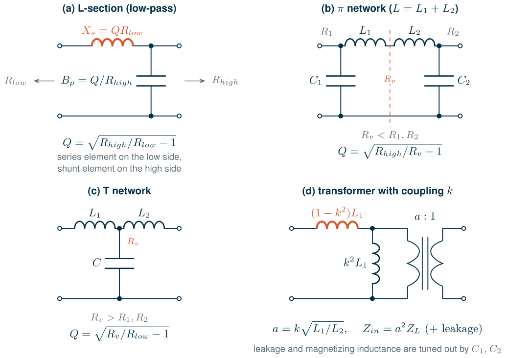
The simplest matching network has two reactances: a series element on the low-resistance side and a shunt element on the high-resistance side (Figure 8.1a). The series reactance \(X_s\) adds to \(R_{low}\) to form an impedance whose parallel equivalent is \(R_{high}\); the shunt susceptance \(B_p\) cancels the reactive part. Both conditions together give the L-section’s design equations [7, 6]:
Key equation · The L-section
\[Q = \sqrt{\frac{R_{high}}{R_{low}} - 1}, \qquad X_s = Q\,R_{low}, \qquad B_p = \frac{Q}{R_{high}}. \tag{8.3}\]
\(Q\) is the quality factor of both branches at the centre frequency, \(X_s/R_{low} = B_p R_{high}\). Once the ratio is fixed, so is \(Q\): an L-section has no free parameter. The series element can be an inductor and the shunt a capacitor (a low-pass L-section, which also attenuates harmonics) or the reverse (a high-pass L-section, whose series capacitor also blocks DC).
Bandwidth
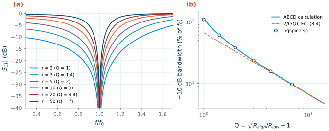
The L-section is a resonant circuit, and its \(Q\) sets its bandwidth. Terminated at both ends, the network’s loaded Q is \(Q/2\) and its 3 dB bandwidth about \(2f_0/Q\). The bandwidth that matters for a match is narrower: where \(\vert S_{11}\vert\) stays below −10 dB, \(\vert S_{21}\vert^2 \ge 0.9\), a third of the 3 dB bandwidth,
\[B_{-10\,\mathrm{dB}} \approx \frac{2}{3}\,\frac{f_0}{Q} \qquad (Q \gtrsim 2). \tag{8.4}\]Figure 8.2 checks Eq. (8.4) with ngspice sp for L-sections from 50 Ω down to 25, 16.7, 10, 5, 2.5 and 1 Ω at 2.44 GHz. Above \(Q\) = 2 the approximation is within 12 % of the simulation: 23.6 % against 22.2 % for a ratio of 10, 9.63 % against 9.52 % for a ratio of 50. Below \(Q \approx 2\) the band is wider than the formula: a ratio of 2 (\(Q\) = 1) is matched to better than −10 dB from 0.732 to 3.40 GHz, 109 % of \(f_0\). A large transformation ratio means a high Q and a narrow band; the only way around it is more sections (Section 8.7).
sp. (b) −10 dB bandwidth against Q: ngspice, an ABCD calculation and Eq. (8.4).8.3 π and T networks and bandwidth
An L-section cannot choose its Q. Adding a third element can: a π network (Figure 8.1b) is two L-sections back to back, the first transforming \(R_{high}\) down to a virtual resistance \(R_v\) below both terminations, the second transforming \(R_v\) up to \(R_{low}\). A T network (Figure 8.1c) does the same through an \(R_v\) above both. The designer picks \(Q\), and the network follows:
\[\pi:\ R_v = \frac{R_{high}}{1 + Q^2},\quad Q_1 = \sqrt{\frac{R_{low}}{R_v} - 1},\quad C_{high} = \frac{Q}{\omega_0 R_{high}},\ C_{low} = \frac{Q_1}{\omega_0 R_{low}},\ L = \frac{(Q + Q_1)R_v}{\omega_0} \tag{8.5}\] \[T:\ R_v = R_{low}(1 + Q^2),\quad Q_2 = \sqrt{\frac{R_v}{R_{high}} - 1},\quad L_{low} = \frac{Q R_{low}}{\omega_0},\ L_{high} = \frac{Q_2 R_{high}}{\omega_0},\ C = \frac{Q + Q_2}{\omega_0 R_v} \tag{8.6}\]A higher \(Q\) narrows the band, which is sometimes wanted: a low-pass π or T attenuates the harmonics of a power amplifier more than an L-section does. The course transmitter needs this. Its second harmonic, at 4.88 GHz, falls in the band of its own VCO (4.80–4.97 GHz, Chapter 5), and it must not reach the antenna.
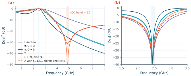
Figure 8.3 compares five networks from \(R_{opt}\) = 10.6 Ω to 50 Ω, simulated with ideal elements; Table 8.1 lists them. The L-section (\(Q\) = 1.93, 1.33 nH and 2.52 pF) is 39.7 % wide but attenuates the second harmonic only 8.8 dB more than the fundamental. A π with \(Q\) = 3 raises this 2f0 rejection to 18.9 dB and halves the bandwidth (20.9 %); a π with \(Q\) = 5 reaches 25.6 dB in 10.3 %. A T with \(R_v\) = 100 Ω behaves like the π with \(Q\) = 3 (18.4 dB, 22.0 %) but needs 5.27 nH of inductance instead of 1.32 nH.
A harmonic trap does better. Replace the shunt capacitor \(C\) of the L-section by a series \(L_t C_t\) that resonates at \(2f_0\). At \(2f_0\) it shorts the output; at \(f_0\) it must still look like \(C\). With \(\omega_t = 2\omega_0\), its reactance at \(\omega_0\) is \(\omega_0 L_t - 4\omega_0 L_t = -3\omega_0 L_t\), so
\[L_t = \frac{1}{3\omega_0^2 C}, \qquad C_t = \frac{3C}{4}. \tag{8.7}\]For \(C\) = 2.52 pF: \(L_t\) = 0.564 nH and \(C_t\) = 1.89 pF. This is design A (Figure 8.4a). With ideal elements its rejection at 4.88 GHz is limited only by numerical precision, and its band, 30.1 %, is still wider than that of the π with \(Q\) = 3.
sp.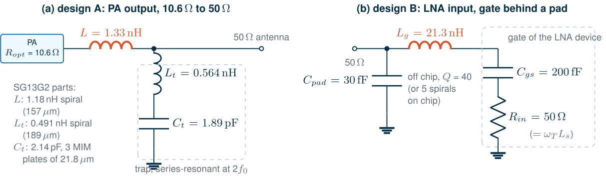
8.4 Matching on the Smith chart
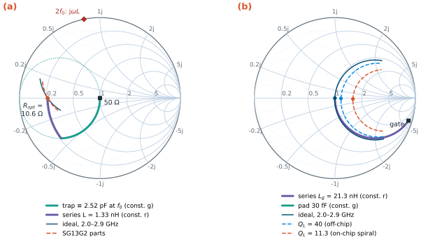
Equations give the element values; the Smith chart shows why a network works and where it can go wrong. Chapter 3 introduced the rules (Table 3.2) [44]: on the impedance chart a series reactance moves a point along its circle of constant resistance \(r\), clockwise for an inductor; on the admittance chart (the same chart turned by 180°) a shunt susceptance moves it along its circle of constant conductance \(g\), clockwise for a capacitor. A lumped match is a path of such arcs from the load to the centre, or, as here, from 50 Ω to the impedance the device wants.
Worked example 8.2 · Design A on the Smith chart
Look from the PA towards the antenna (Figure 8.5a). Start at the antenna, \(z\) = 1 at the centre of a 50 Ω chart. At \(f_0\) the trap is a capacitor of 2.52 pF, a normalized susceptance \(b = \omega_0 C Z_0\) = 1.93: the point moves clockwise along the circle \(g\) = 1 to \(y = 1 + j1.93\), that is \(z\) = 0.212 − j0.409. Now the series inductor, 20.4 Ω or \(x\) = 0.409, moves it along the circle \(r\) = 0.212 up to the real axis: \(z\) = 0.212, or 10.6 Ω. The ngspice curves trace the input impedance from 2.0 to 2.9 GHz through the target. At \(2f_0\) the trap shorts the antenna node and the PA sees only \(j2\omega_0 L\), a point on the rim of the chart: no power can reach the 50 Ω load there.
The chart also shows the bandwidth. The longer the arcs, the more the end point moves when the frequency changes: a network that goes far around the chart (a high Q) is narrow. Paths that pass close to the rim, where \(r\) or \(g\) is small, carry large circulating currents and voltages, and are lossy with real components.
Design B (Figure 8.5b) matches 50 Ω to the gate of an LNA device: \(C_{gs}\) = 200 fF in series with the 50 Ω real part that inductive source degeneration provides (\(\omega_T L_s\), Chapter 9), behind a pad of 30 fF (an 80 µm × 80 µm TopMetal2 pad over a Metal1 shield: 23.8 fF of parallel plate, plus fringing). The gate’s reactance is 326 Ω, \(z_g\) = 1 − j6.52, close to the rim. A series inductor moves it along \(r\) = 1 almost to the centre, and the pad, a small susceptance, finishes the job: \(L_g\) = 21.3 nH. The match is a series resonance with a loaded Q of \(\omega_0 L_g/(100\ \Omega)\) = 3.27, and its −10 dB band runs from 2.32 to 2.57 GHz (10.2 %), three times the 3.42 % of the BLE band.
8.5 Loss in matching networks
Real inductors have a Q of about 10 at 2.4 GHz (Chapter 7), and a matching network multiplies their loss by its own Q. In an L-section the current through the series inductor is the current into \(R_{low}\), so its series resistance \(X_s/Q_L = Q R_{low}/Q_L\) dissipates \(Q/Q_L\) times the delivered power; the shunt capacitor, which sees the voltage across \(R_{high}\), adds \(Q/Q_C\):
Key equation · Insertion loss of an L-section
\[IL \approx 10\log_{10}\!\left(1 + \frac{Q}{Q_L} + \frac{Q}{Q_C}\right)\ \mathrm{dB}. \tag{8.8}\]
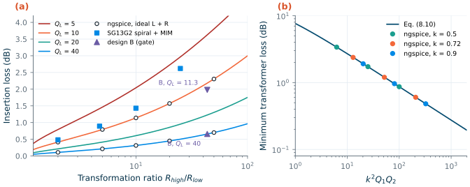
The ratio of the network’s Q to the components’ Q is what counts. Figure 8.6a plots Eq. (8.8) for \(Q_C \to \infty\). With ideal elements and a series resistance for \(Q_L\), ngspice agrees with it exactly (to 4 × 10⁻⁶ dB). With an inductor of \(Q_L\) = 10, a ratio of 2 costs 0.414 dB, a ratio of 20 already 1.57 dB; an off-chip inductor with \(Q_L\) = 40 brings these to 0.107 and 0.449 dB.
With SG13G2’s parts. We rebuilt L-sections from 50 Ω to 25, 10.6, 5 and 2 Ω with the EM-fitted spirals of Chapter 7 (tools/figs/_ch07_inductor.py) and cap_rfcmim capacitors split into plates of at most 25 µm with 10 µm feeds, and re-tuned each to a perfect match at 2.44 GHz. The blue squares of Figure 8.6a: 0.482, 0.892, 1.43 and 2.62 dB. They lie above Eq. (8.8) with the spirals’ Q (9.95 for the 1.25 nH spiral of the 10.6 Ω match) because a matched network must also absorb the inductor’s resistance: the spiral’s 1.90 Ω in series with 10.6 Ω forces a higher Q, 2.16 instead of 1.93 (the larger shunt capacitor of the re-tuned network shows it). Eq. (8.8) with the Q of the network as built, and the capacitor’s Q of 298, gives 0.880 dB, within 0.02 dB of the simulation; for the 2 Ω match the Q rises from 4.90 to 6.66 and the estimate matches to 0.01 dB. The capacitors matter little: MIM plates of this size have a Q near 300 at 2.44 GHz.
What this means for your design
At 2.4 GHz with on-chip spirals, every unit of network Q costs about 0.4 dB. The PA’s 50 Ω to 10.6 Ω match costs 0.892 dB, so the PA must deliver about +10.9 dBm for +10 dBm at the antenna, 23 % more power and a lower PAE. Keep the transformation ratio small (a higher supply raises \(R_{opt}\)), and spend extra Q only where it buys something, such as harmonic rejection.
The PA match with real parts. Table 8.1 lists the five PA networks built with SG13G2 parts. The loss grows with the network’s Q: 0.892 dB for the L-section, 1.43 dB for the π with \(Q\) = 3 (Eq. (8.8) with \(Q + Q_1\) = 4.06 and \(Q_L\) = 9.97 predicts 1.48 dB), 2.77 dB for the π with \(Q\) = 5. The losses also lower the networks’ effective Q: in the π with \(Q\) = 3 the virtual resistance is only 5 Ω, and the spiral adds 2 Ω to it, so the re-tuned network is wider (33.1 %) and rejects less (14.3 dB) than the ideal one. Design A costs 1.26 dB: 0.37 dB more than the plain L-section, for 30.1 dB of 2f0 rejection. Its trap spiral has a Q of 8.30 at f0, where it carries the shunt current, and 13.8 at 2f0, where its resistance sets the depth of the notch. Built from SG13G2 parts its values move a little: a 1.18 nH spiral (DC inductance; 157 µm), a 0.491 nH spiral (189 µm) and 2.14 pF in three MIM plates.
Table 8.1. Matching networks of this chapter at their design frequency (ngspice sp; "SG13G2": EM-fitted spirals and cap_rfcmim, re-tuned to a perfect match; area: spirals' outer diameter squared plus MIM area).
| Network | Inductance | −10 dB BW, ideal / SG13G2 | 2f0 rejection, ideal / SG13G2 | Loss (SG13G2) | Area |
|---|---|---|---|---|---|
| PA: L-section, 10.6 → 50 Ω | 1.33 nH | 39.7 % / 42.4 % | 8.8 / 8.78 dB | 0.892 dB | 0.027 mm² |
| PA: π, Q = 3 | 1.32 nH | 20.9 % / 33.1 % | 18.9 / 14.3 dB | 1.43 dB | 0.031 mm² |
| PA: π, Q = 5 | 0.894 nH | 10.3 % / 17.3 % | 25.6 / 21.3 dB | 2.77 dB | 0.034 mm² |
| PA: T, Rv = 100 Ω | 5.27 nH | 22.0 % / 21.4 % | 18.4 / 20.5 dB | 1.95 dB | 0.073 mm² |
| PA: design A, L + 2f0 trap | 1.90 nH | 30.1 % / 33.7 % | > 100 / 30.1 dB | 1.26 dB | 0.062 mm² |
| PA: transformer, k = 0.72 | 0.337 + 1.49 nH | 29.6 % / 36.2 % | 0.65 / 2.17 dB | 1.34 dB | – |
| LNA: design B, Lg (Q = 40 / 11.3) | 21.3 nH | 10.2 % / 10.7 % (Q = 40) | – | 0.658 / 1.98 dB | off chip |
| 50 GHz: single stub (TopMetal2) | 424 µm of line | 33.6 % / 36.1 % | – | 0.717 dB | – |
| 50 GHz: line + λ/4 (TopMetal2) | 1112 µm of line | 18.1 % / 20.3 % | – | 1.21 dB | – |
Matching to a high impedance. The gate of design B is a capacitor with a small series resistance, and its parallel equivalent is large: 200 fF in series with 50 Ω is \(R_p = R(1 + Q^2)\) = 2.18 kΩ in parallel with a capacitor, at \(Q\) = 6.52. Matching 50 Ω to it is a transformation ratio of 43.5, and Eq. (8.8) applies with \(Q\) = 6.52: the violet triangles of Figure 8.6a. An off-chip gate inductor with \(Q_L\) = 40 has 8.18 Ω of series resistance and costs 0.658 dB; an on-chip one with the 11.3 of the best Chapter 7 spiral would cost 1.98 dB, and the 21.3 nH would need five spirals in series, since the fitted family stops at 4.94 nH. A loss in front of the LNA adds directly to its noise figure, which is why the course LNA puts its gate inductor off chip (Chapter 9).
8.6 Transformer and transmission-line matching
Transformers
An ideal transformer with \(n\) times more turns on its secondary transforms an impedance by \(n^2\), at every frequency. An on-chip transformer is far from ideal: its windings have finite inductance, and only part of their flux is shared, \(k\) = 0.72 for the stacked transformer of Chapter 7. Figure 8.1d shows the equivalent circuit: an ideal transformer behind a series leakage inductance \((1-k^2)L_1\) and a shunt magnetizing inductance \(k^2L_1\), with the ratio
\[a = k\sqrt{L_1/L_2}, \qquad Z_{in} = a^2 Z_L \ \text{(with the inductances tuned out)}. \tag{8.9}\]Capacitors across both windings tune out the reactances; then the transformer behaves like a double-tuned band-pass filter. Its loss depends on just one number [108, 109]:
Key equation · Maximum efficiency of a transformer
\[\eta_{max} = \frac{x}{\left(1 + \sqrt{1 + x}\right)^2}, \qquad x = k^2 Q_1 Q_2, \tag{8.10}\]reached when the secondary resonates and its load sets its loaded Q to \(Q_s = Q_2/\sqrt{1 + x}\).
Derivation · Eq. (8.10)
Let the secondary loop (winding resistance \(R_2 = \omega L_2/Q_2\), inductance \(L_2\) and the tuned load, which presents \(R' - j\omega L_2\)) resonate. Its efficiency is \(\eta_2 = R'/(R_2 + R')\). The primary current \(I_1\) induces \(j\omega M I_1\), so the secondary reflects \(R_{refl} = \omega^2 M^2/(R_2 + R')\) into the primary, whose efficiency is \(\eta_1 = R_{refl}/(R_1 + R_{refl})\). With \(t = R'/R_2\) and \(x = \omega^2M^2/(R_1R_2) = k^2Q_1Q_2\),
\[\eta = \eta_1\eta_2 = \frac{x\,t}{(1 + t)(1 + t + x)},\]which is largest for \(t = \sqrt{1 + x}\); substituting gives Eq. (8.10). A secondary load \(R_L\) in parallel with \(C_2\) presents \(R' = R_L/(1 + Q_s^2)\) and \(X' = R_L Q_s/(1 + Q_s^2)\), with \(Q_s = \omega C_2 R_L\); resonance (\(X' = \omega L_2\)) and \(t = \sqrt{1+x}\) together give \(Q_s = Q_2/\sqrt{1 + x}\).
Figure 8.6b checks Eq. (8.10) with ngspice for \(k\) = 0.5, 0.72 and 0.9 and winding Q of 5, 10 and 20: every point falls on the curve. For our PA match (Figure 8.7a), the optimum loading gives \(L_2\) = 1.49 nH and \(C_2\) = 2.00 pF on the antenna side; the primary must then be \(L_1\) = 0.337 nH (one turn, like T1 of Chapter 7) with \(C_1\) = 7.73 pF, a turns ratio of about 2.1. With the Q of Chapter 7’s spirals at 2.44 GHz (8.0 for the one-turn primary, 10.0 for the secondary), \(x\) = 41.5 and the loss is 1.34 dB, as Eq. (8.10) predicts. That is more than the L-section’s 0.892 dB: at a ratio of 4.7 a transformer does not pay for itself in loss. It earns its place for other reasons: it isolates DC, feeds the collector through a centre tap, converts a differential PA to a single-ended antenna (a balun), and combines several PA cells [108, 101]. Its bandwidth is wide (36.2 %), but it hardly filters: its 2f0 rejection is 2.17 dB.
Transmission lines at millimetre waves
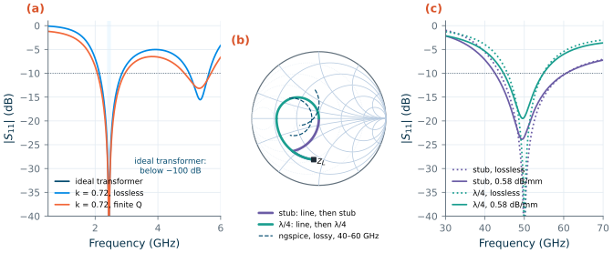
At 50 GHz a quarter wavelength on the TopMetal2 microstrip of Chapter 7 (47.8 Ω, \(\varepsilon_{eff}\) = 3.73, 0.583 dB/mm) is 776 µm, and lines become the natural matching elements [8, 10]. As in Chapter 3, take the load 20 Ω + 79.6 fF (\(z_L\) = 0.4 − j0.8 at 50 GHz). For the lossy simulation we model the line with ngspice’s LTRA element, using \(R'\) = 6.42 Ω/mm, \(L'\) = 0.308 nH/mm and \(C'\) = 0.135 pF/mm derived from the EM results (constant \(R'\), so the skin effect’s growth with frequency is left out).
Single stub. A line of length \(d\) rotates the load on a circle of constant \(\vert\Gamma\vert\) until it reaches the circle \(g\) = 1; a shunt stub then cancels the susceptance (Figure 8.7b). Here \(d\) = 139 µm (16.2°) brings the admittance to \(y\) = 1.00 + j1.61, and a short-circuited stub of 285 µm (33.0°) cancels it. A shorted stub is easy on chip (a via to the Metal1 ground) and carries the collector bias at the same time.
Quarter-wave transformer. A line of 370 µm brings the load to the real axis at 11.3 Ω, and a λ/4 section of \(Z_1 = \sqrt{50 \times 11.3}\) = 23.7 Ω transforms that to 50 Ω. A 23.7 Ω microstrip is 49.2 µm wide (Hammerstad–Jensen [105], scaled to the EM result of Chapter 7), with \(\varepsilon_{eff}\) = 4.08, so the section is 742 µm long; we assume the same loss per millimetre as the 16 µm line.
Figure 8.7c and Table 8.1 compare the two. The stub match uses 424 µm of line, is 36.1 % wide and loses 0.717 dB; the quarter-wave match uses 1112 µm, is 20.3 % wide and loses 1.21 dB. The stub loses far more than its 139 µm of series line alone (0.081 dB): the stub and the line near the load carry standing waves, so their current, and their loss, is higher than in a matched line. At millimetre waves the shortest network with the lowest standing-wave ratio wins; Chapter 17 designs the 50 GHz amplifier’s matches this way and checks them with EM simulation.
sp.8.7 Broadband matching and its limits
Section 8.2 showed that a high transformation ratio makes an L-section narrow. More sections help: two L-sections through an intermediate resistance \(\sqrt{R_{high}R_{low}}\) each have a lower Q, and a cascade of many approaches a tapered line. For a purely resistive load there is no limit. A reactive load is different. Bode [20] and Fano [107] showed that no lossless network, however complex, can match a load with stored energy over an arbitrary band. For a load \(R\) in series with \(C\), such as the gate of design B,
Key equation · The Bode–Fano limit (series RC load)
\[\int_0^\infty \frac{1}{\omega^2}\,\ln\frac{1}{\vert\Gamma(\omega)\vert}\,d\omega \le \pi R C \quad\Rightarrow\quad \frac{\Delta\omega}{\omega_0} \le \frac{\pi}{Q\,\ln(1/\Gamma_m)}, \tag{8.11}\]where the right-hand form holds for \(\vert\Gamma\vert = \Gamma_m\) inside a band \(\Delta\omega\) around \(\omega_0\) and \(\vert\Gamma\vert\) = 1 outside, and \(Q = 1/(\omega_0RC)\). (For a parallel RC the integral of \(\ln(1/\vert\Gamma\vert)\) itself is bounded by \(\pi/RC\).)
The integral is a budget. A match can spend it on a narrow band with a deep null, or on a wide band with a modest return loss, but not more. For the gate of design B, \(Q\) = 6.52, so a 10 dB return loss (\(\Gamma_m\) = 0.316) can be held over at most 41.8 % of \(f_0\), 1020 MHz.
Figure 8.8 shows how close real networks come. We optimized ladders of one and two resonators for the widest −10 dB band (differential evolution, ideal elements) and simulated them with ngspice. The single series \(L_g\) of design B covers 10.2 %. Adding a shunt resonator at the pad (0.962 nH in parallel with 4.42 pF, which absorbs the pad’s 30 fF) widens it to 14.7 %, and adding also a 3.13 nH series inductor at the input, which lets the network choose its internal impedance level, to 24.9 % (2.16–2.76 GHz), with the equal-ripple response typical of such optimized matches. All three networks spend the same budget: their Bode–Fano integral, computed numerically from 1 MHz to 10 THz, equals \(\pi RC\) to within 0.1 %. The extra elements do not create matching; they move it from the deep null into the band.
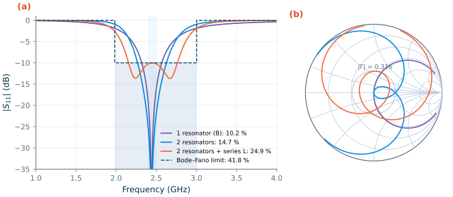
sp. (a) |S11| and the Bode–Fano limit of Eq. (8.11) (dashed: the ideal rectangular response). (b) The same on the Smith chart, 1.5–3.6 GHz; dotted: |Γ| = 0.316.The course radio needs only the 3.42 % of the BLE band, which a single resonator covers three times over. Broadband matching matters for multi-band and wideband receivers, which therefore often avoid resonant matches altogether and use resistive feedback or common-gate inputs whose real input resistance does not need a reactance to be tuned out (Chapter 9). Every extra element also adds loss (Section 8.5), so a wideband match on chip pays twice.
Common pitfall · Designing with ideal elements and forgetting to re-tune
A network designed with ideal elements and then built with real spirals is no longer matched: the spiral’s resistance adds to the low-impedance side and its effective inductance differs from its DC value. In this chapter the re-tuning moved the PA L-section’s capacitor from 2.52 to 2.81 pF and design A’s trap capacitor from 1.89 to 2.14 pF. Always re-tune with the real component models, and judge a network by its loss after re-tuning.
Try it · The matching script
Every number in this chapter comes from
tools/figs/ch08_matching.py(run it inside IIC-OSIC-TOOLS;python3 tools/figs/ch08_matching.py pa lossfor some parts). Three experiments: (1) ChangeVCCto 1.0 V: how much do \(R_{opt}\) and the loss of design A change? (2) Inpa_specs(), move the trap to the PA side of the series inductor (the drain); compare its rejection and loss with design A. (3) Inbf_net(), add a third resonator and re-runbf --resim(several minutes): how close does the band come to 41.8 %?
- Match for power at the chip’s ports, for noise at the LNA’s input, and for the load line at the PA’s output: Ropt = (VCC − Vknee)²/2Pout is 10.6 Ω for +10 dBm from an npn13G2 at 0.8 V. Inside the chip, do not match.
- An L-section’s Q is fixed by its ratio, Q = √(Rhigh/Rlow − 1), and its −10 dB bandwidth is about 2f0/3Q. π and T networks choose a higher Q through a virtual resistance.
- On the Smith chart a series element moves along a circle of constant r, a shunt element along a circle of constant g; long arcs near the rim mean a narrow, lossy network.
- A network multiplies the loss of its components by its Q: IL ≈ 10 log(1 + Q/QL + Q/QC). With SG13G2 spirals the PA’s 10.6 → 50 Ω L-section loses 0.892 dB; a trap at 2f0 (design A) adds 0.37 dB for 30.1 dB of second-harmonic rejection, much better than a high-Q π.
- A transformer’s loss depends only on k²Q1Q2 (1.34 dB for k = 0.72 and Q ≈ 9); at 50 GHz a short single-stub match on TopMetal2 loses 0.717 dB against 1.21 dB for a quarter-wave transformer.
- The Bode–Fano limit caps the bandwidth of any match of a reactive load: 41.8 % at −10 dB for the LNA gate, of which one resonator uses 10.2 % and two 24.9 %.
Further reading
- D. M. Pozar, Microwave Engineering [8]: L-section, stub, quarter-wave and multi-section matching, and the Bode–Fano criterion, with many worked problems; G. Gonzalez [9] for matching amplifiers on the Smith chart.
- T. H. Lee [7]: the L, π and T networks and their Q from an IC designer’s point of view.
- S. C. Cripps [13]: the load line, Ropt and the output networks of power amplifiers.
- R. M. Fano [107] and H. W. Bode [20]: the original theory of the limits of broadband matching.
- I. Aoki et al. [108] and K. H. An et al. [109]: transformer-based matching and power combining for fully integrated PAs, including the efficiency of a transformer with finite k and Q.