Chapter 4
Noise and Linearity
A receiver must hear a signal of a few picowatts while a transmitter next door shouts with milliwatts. Noise sets the weakest signal it can detect; nonlinearity sets the strongest it can handle. This chapter defines the two numbers that capture them, the noise figure and the intercept point, simulates both on two SG13G2 amplifier stages, and turns them into the noise and linearity budget of the course receiver.
- Describe thermal, shot and flicker noise, and express the noise of a transistor as an equivalent noise resistance.
- Define the noise figure with a 290 K source, compute it by hand for a simple stage, and simulate it with ngspice’s S-parameter noise analysis.
- Apply the Friis formula to a cascade, and derive a receiver’s noise-figure budget from its sensitivity target.
- Model a nonlinear stage as a power series, and predict its harmonics, 1 dB compression point, IIP3 and IIP2; measure them with harmonic balance in Xyce.
- Explain blocking, desensitization and cross-modulation, and compute the cascaded IIP3 and spurious-free dynamic range of a receiver.
Contents
- 4.1 Noise sources and the noise floor
- 4.2 Noise figure and noise temperature
- 4.3 Cascades: the Friis formula
- 4.4 Sensitivity
- 4.5 Harmonics and gain compression
- 4.6 Intermodulation and intercept points
- 4.7 Blocking, desensitization and cross-modulation
- 4.8 Cascaded linearity and dynamic range
- Further reading
4.1 Noise sources and the noise floor
Every resistor is a noise generator. The thermal motion of its carriers makes a random voltage across it, with a spectrum that is flat (white) far beyond any radio frequency. Johnson measured it and Nyquist explained it in 1928 [55, 56]: in a bandwidth \(\Delta f\), a resistance \(R\) at the absolute temperature \(T\) has a mean-square open-circuit noise voltage
\[\overline{v_n^2} = 4kTR\,\Delta f. \tag{4.1}\]A 50 Ω resistor at 290 K gives 0.895 nV/√Hz. Connected to a matched load, it delivers a quarter of \(\overline{v_n^2}/R\), the available noise power
\[P_n = kTB, \tag{4.2}\]in a bandwidth \(B\), whatever the value of \(R\). At the reference temperature \(T_0\) = 290 K, \(kT_0\) is −174.0 dBm/Hz, the noise floor of every matched system that Chapter 1 introduced. In the 1 MHz noise bandwidth of the course radio it is −114.0 dBm.
Two other mechanisms matter in transistors. When carriers cross a potential barrier independently of each other, as in a pn junction, the current fluctuates around its mean \(I\): this is shot noise [57],
\[\overline{i_n^2} = 2qI\,\Delta f. \tag{4.3}\]At low frequencies, every device also shows flicker noise, whose spectral density rises as \(1/f\). Carriers trapped and released by defects at the oxide interface, and fluctuations of their mobility, cause it [58, 59]. It is strong in MOSFETs, whose channel runs along the oxide, and weak in bipolar transistors, whose current flows through the bulk. The frequency at which flicker noise equals the white noise is the flicker corner. A 2.4 GHz amplifier does not see flicker noise directly, but mixers and oscillators translate it to radio frequencies (Chapters 10 and 11).
In a saturated MOSFET the channel behaves as a resistive strip, and its thermal noise appears at the drain as a current with a white spectral density \(4kT\gamma g_m\); \(\gamma\) is 2/3 for a long channel and larger for a short one [60, 61]. The collector current of a bipolar transistor carries the shot noise \(2qI_C\):
\[\overline{i_d^2} = 4kT\gamma g_m\,\Delta f + \frac{K_f\,g_m^2}{C_{ox}WL}\,\frac{\Delta f}{f}, \qquad \overline{i_c^2} = 2qI_C\,\Delta f. \tag{4.4–4.5}\]To compare devices, refer the noise to the input. Divide the output current noise by \(g_m^2\), add the thermal noise of the resistances in series with the input (the gate resistance \(R_g\); the base and emitter resistances \(r_b\) and \(r_e\)), and express the result as the resistance whose thermal noise is the same, the equivalent noise resistance \(R_n\):
Key equation · Input noise of a transistor
\[\overline{v_n^2} = 4kTR_n\,\Delta f, \qquad R_n = R_g + \frac{\gamma}{g_m}\ \ \text{(MOSFET)}, \qquad R_n = r_b + r_e + \frac{1}{2g_m}\ \ \text{(bipolar)} \tag{4.6}\]For the bipolar transistor, \(2qI_C/g_m^2 = 4kT/(2g_m)\) with \(g_m = qI_C/kT\).
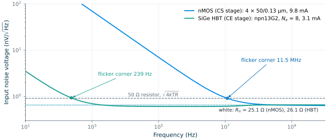
The two transistors of this chapter are biased for the same transconductance at 2.44 GHz: an nMOS made of four parallel 50/0.13 µm sg13_lv_nmos devices (ngspice model with rfmode=1), \(g_m\) = 74.6 mS at 9.81 mA, and an npn13G2 HBT with eight emitter fingers, \(g_m\) = 74.3 mS at 3.08 mA. The HBT needs a third of the current: 24.1 S/A against 7.6 S/A. Figure 4.1 shows their input noise from ngspice’s noise analysis. Above a few hundred megahertz both are white, at 0.645 and 0.658 nV/√Hz, less than a 50 Ω resistor: Rn = 25.1 Ω for the nMOS and 26.1 Ω for the HBT. The nMOS number splits into \(\gamma/g_m\) = 12.2 Ω, with \(\gamma\) = 0.91 from a simulation without the RF sub-circuit, and a gate resistance of 12.9 Ω that the RF model adds. For the HBT, the model card’s \(r_b\) = 15.0 Ω and \(r_e\) = 3.56 Ω and \(1/(2g_m)\) = 4.2 Ω (with \(g_m = qI_C/kT\) = 119 mS) add up to 22.7 Ω, 13 % less than simulated. The flicker corners differ by almost five decades: 11.5 MHz for the nMOS, 239 Hz for the HBT.
4.2 Noise figure and noise temperature
The noise of a block matters only in comparison with the noise that arrives with the signal. The noise factor \(F\) is the ratio of the signal-to-noise ratios at the input and output, with the source resistance at \(T_0\) = 290 K [62, 187]. If the block has available gain \(G_A\) and adds a noise power \(N_{added}\) at its output, the input SNR is \(S/kT_0B\) and the output SNR is \(G_AS/(G_AkT_0B + N_{added})\), so
\[F = \frac{\mathrm{SNR}_{in}}{\mathrm{SNR}_{out}} = 1 + \frac{N_{added}}{G_AkT_0B}, \qquad \mathrm{NF} = 10\log_{10}F. \tag{4.7}\]A noiseless block has \(F\) = 1, an NF of 0 dB. The noise temperature expresses the added noise as the temperature to which the source would have to be heated to produce it at the input,
\[T_e = (F - 1)\,T_0, \tag{4.8}\]which is the natural unit for very quiet amplifiers: an NF of 0.5 dB is a \(T_e\) of 35 K. The 290 K is a convention, close to room temperature, that makes \(kT_0\) a round −174 dBm/Hz. An NF also depends on the source impedance, so a noise figure without “290 K” and “50 Ω” (or the actual source impedance) is incomplete.
A matched attenuator at \(T_0\) is the simplest example. It is a network of resistors at \(T_0\) matched to the source, so its available output noise is \(kT_0B\), the same as the source’s; but its available gain is \(1/L\). From Eq. (4.7), \(F = L\): a 3 dB attenuator has an NF of 3 dB, and every decibel of loss in a filter, switch or cable in front of a receiver adds a decibel to its NF. At a physical temperature \(T\) the noise factor becomes \(1 + (L-1)\,T/T_0\), 3.08 dB at 27 °C.
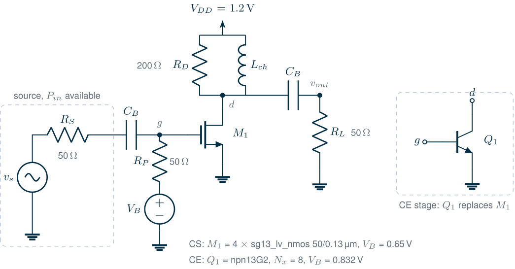
Figure 4.2 shows the two amplifier stages that the rest of the chapter studies. Each transistor drives a 200 Ω resistor \(R_D\), in parallel with an ideal choke that carries the bias current, and a 50 Ω load. A 50 Ω resistor \(R_P\) from the input to the bias voltage matches the input to the source over a wide band: \(S_{11}\) is −15.1 dB for the common-source (CS) stage and −27.3 dB for the common-emitter (CE) stage at 2.44 GHz, and the gains \(\vert S_{21}\vert^2\) are 8.22 and 9.38 dB. These are not good low-noise amplifiers (Chapter 9 designs those), but they are the simplest stages with a well-defined noise figure in a 50 Ω system.
The noise factor of this stage follows from Eq. (4.7) by adding up the noise sources referred to the input:
Key equation · Noise factor of a resistively terminated stage
\[F = 2 + \frac{4R_n}{R_S} + \frac{4}{g_m^2R_DR_S} \tag{4.9}\]The source contributes 1, the termination resistor \(R_P = R_S\) another 1, the transistor \(4R_n/R_S\) and the load resistor the last term.
Derivation · Noise factor of the resistively terminated stage
With \(R_P = R_S\), the gate sees half the source voltage, behind \(R_S/2\). Refer every noise source to a voltage at the gate and compare it with the source’s own noise there, \(4kTR_S\,(1/2)^2 = kTR_S\) (per hertz):
- \(R_P\): its noise current \(4kT/R_P\) flows into \(R_S \parallel R_P = R_S/2\), giving \(kTR_S^2/R_P\), a ratio \(R_S/R_P = 1\).
- The transistor: \(4kTR_n\) in series with the gate, a ratio \(4R_n/R_S\).
- \(R_D\): its noise current \(4kT/R_D\) at the drain, divided by \(g_m^2\), gives \(4kT/(g_m^2R_D)\), a ratio \(4/(g_m^2R_DR_S)\).
The noise of the load \(R_L\) is not counted: the noise figure counts the noise a block adds, and the load belongs to the next stage. Adding 1 for the source gives Eq. (4.9). The input capacitance and the transistor’s output resistance are neglected.
For the CS stage, \(4R_n/R_S\) = 2.01 and the \(R_D\) term is 0.072; for the CE stage, 2.09 and 0.072. With the correction for 300 K parts and a 290 K source (see the pitfall below), Eq. (4.9) gives NF = 6.22 dB for the CS stage and 6.31 dB for the CE stage. ngspice’s S-parameter noise analysis gives 6.22 and 6.33 dB at 2.44 GHz (Figure 4.3a), flat within 0.1 dB from 0.5 to 6 GHz. The breakdown shows where the noise comes from: half of it is the source and the termination resistor, which is why a resistively matched stage can never reach an NF below 3 dB. The transistor adds almost as much again. In the nMOS, half of that is the gate resistance: without the RF sub-circuit the same stage has an NF of 4.93 dB.
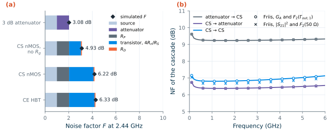
sp noise analysis (diamonds, with NF in dB); "no Rg": the nMOS model without its RF sub-circuit. (b) Noise figure of three two-stage cascades simulated as a whole (lines) and from the Friis formula, Eq. (4.11), with the per-stage S-parameters and noise parameters (circles: available gain and F2 for the output impedance of stage 1; crosses: |S21|2 and F2 for 50 Ω). All noise figures for a 290 K source; tt, 27 °C.The noise factor of a two-port depends on its source impedance. Rothe and Dahlke showed that four numbers describe it for every source [63, 64]: the minimum noise factor \(F_{min}\), reached for an optimum source reflection coefficient \(\Gamma_{opt}\), and the noise resistance \(R_n\) that sets how fast \(F\) rises away from it,
\[F = F_{min} + \frac{4R_n}{Z_0}\,\frac{\vert\Gamma_S - \Gamma_{opt}\vert^2}{\left(1 - \vert\Gamma_S\vert^2\right)\vert 1 + \Gamma_{opt}\vert^2}. \tag{4.10}\]ngspice’s sp analysis with the noise flag returns all four (nfmin, rn, sopt, and nf for the 50 Ω source). Our stages have \(\mathrm{NF}_{min}\) = 5.92 dB (CS) and 6.04 dB (CE), only 0.3 dB below their 50 Ω noise figures: the termination resistor already presents nearly the optimum source. Chapter 6 extracts the noise parameters of the bare transistors, and Chapter 9 designs a match that brings \(\Gamma_S\) to \(\Gamma_{opt}\).
Common pitfall · ngspice’s noise figure is not referenced to 290 K
ngspice reports exactly 3.00 dB for a matched 3 dB attenuator, whether the circuit is at −73 °C, 27 °C or 127 °C. It references its noise figure to the circuit temperature, not to \(T_0\), so it never shows the 2.27 dB and 3.75 dB that such an attenuator really has at −73 °C and 127 °C. To get the standard noise figure from a simulation at a temperature \(T\), use \(F = 1 + (F_{sim} - 1)\,T/T_0\). At 27 °C this adds 0.08 dB to 3 dB and 0.1 dB to 6 dB; every noise figure in this chapter is corrected this way.
SG13G2 · The gate resistance of the RF MOSFET model
With
rfmode=1, SG13G2’s MOSFET model switches to an RF parameter set with a non-quasi-static channel, a substrate network and a gate resistance with a fixed part (rgo= 40 Ω) per instance [191]. A single 200 µm instance would therefore have more than 40 Ω of gate resistance, which by Eq. (4.9) alone would add more than 3 (\(4R_g/R_S\)) to the noise factor of our stage. Building it from four parallel instances (m=4), as a layout of four cells would be, divides it by four: the 12.9 Ω extracted above. Chapter 6 looks at fingers, cells and gate resistance in detail.
4.3 Cascades: the Friis formula
A receiver is a chain of blocks (Figure 4.4). Each block amplifies the noise of the blocks before it together with the signal, and adds its own. Referred to the input, the noise a stage adds is divided by the gain in front of it. Friis wrote the result in 1944 [62]:
Key equation · Noise factor of a cascade (Friis)
\[F = F_1 + \frac{F_2 - 1}{G_1} + \frac{F_3 - 1}{G_1G_2} + \dots \tag{4.11}\]\(G_k\) is the available gain of stage \(k\), and \(F_k\) its noise factor for the source impedance it actually sees: the output impedance of the stage before it.
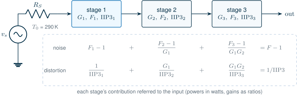
The first stage dominates: its noise enters in full, while the second stage’s is divided by \(G_1\). A good receiver therefore puts a low-noise amplifier with enough gain first, and keeps every lossy element in front of it as short as possible.
Worked example 4.1 · A 3 dB filter before or after the stage
A band filter with 3 dB of loss can go before or after the CS stage (NF 6.22 dB, \(F_1\) = 4.19; \(\vert S_{21}\vert^2\) = 8.22 dB). Before it, the filter is stage 1 with \(F_1 = L\) and \(G_1 = 1/L\), so \(F = L + (4.19 - 1)L = 4.19\,L\): the NF grows by the full 3 dB, to about 9.2 dB. After it, the filter is stage 2 with \(F_2 \approx 2.03\) (its 3 dB of loss at 300 K), and \(F \approx 4.19 + 1.03/6.64 = 4.34\), or 6.38 dB: only 0.16 dB worse than the stage alone.
The simulations of the complete cascades agree: 9.24 dB and 6.40 dB (Figure 4.3b). An antenna filter costs sensitivity decibel for decibel; a filter after the LNA costs almost nothing.
The third cascade of Figure 4.3b, two CS stages in series, shows why Eq. (4.11) insists on available gain and on the actual source impedance. With the 50 Ω noise figure of stage 2 and the insertion gain \(\vert S_{21}\vert^2\) of stage 1, the formula predicts 6.69 dB; the simulation gives 6.84 dB. Stage 1’s output impedance is not 50 Ω but (85.7 − j57.0) Ω, for which stage 2’s NF, from its noise parameters and Eq. (4.10), is 8.06 dB instead of 6.22 dB; and stage 1’s available gain is 9.24 dB, not 8.22 dB. With both corrections, the Friis formula reproduces the simulation of all three cascades to within \(10^{-9}\) dB: it is exact for linear two-ports.
4.4 Sensitivity
The sensitivity of a receiver is the smallest input power at which it still demodulates with the required error rate. The demodulator needs a minimum SNR, \(\mathrm{SNR}_{min}\), in the receiver’s noise bandwidth \(B\); referred to the input, the noise in that bandwidth is \(kT_0B\,F\). In decibels:
Key equation · Sensitivity
\[P_{sens} = -174\ \mathrm{dBm/Hz} + 10\log_{10}B + \mathrm{NF} + \mathrm{SNR}_{min} \tag{4.12}\]
Digital systems usually quote the required \(E_b/N_0\), the energy per bit over the noise spectral density. For a bit rate \(R_b\),
\[\mathrm{SNR} = \frac{E_b}{N_0}\,\frac{R_b}{B}, \tag{4.13}\]and for the course radio, 1 Mb/s in a 1 MHz noise bandwidth, the two are equal. Bluetooth Low Energy defines sensitivity at a bit-error rate of 0.1 % and requires −70 dBm or better [184]; the course radio aims at −90 dBm. Its modulation is Gaussian frequency-shift keying (GFSK) with a Gaussian filter of bandwidth-time product BT = 0.5 and a modulation index of 0.5, the GMSK of Murota and Hirade [65]. The SNR it needs depends on the demodulator. We simulated the simplest one, a differential (discriminator) detector that decides each bit from the phase change over one bit period [66], after a fourth-order Butterworth channel filter with a 1 MHz noise bandwidth: a Monte Carlo run of 2 × 105 bits per point in Python (Figure 4.5a). The 0.1 % bit-error rate needs an SNR of 12.3 dB.
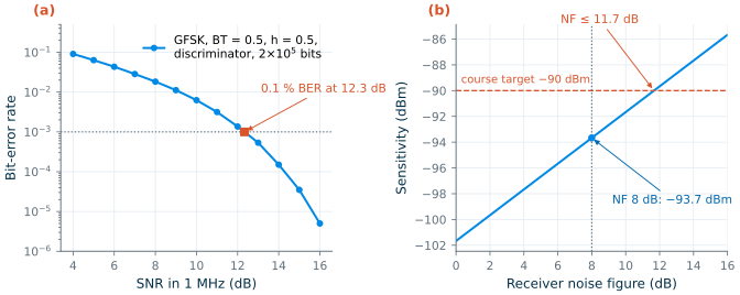
With \(B\) = 1 MHz and an NF of 8 dB, the course specification, Eq. (4.12) gives a sensitivity of −93.7 dBm. Turned around, the −90 dBm target allows an NF of up to 11.7 dB (Figure 4.5b). The specification of 8 dB keeps a margin of 3.7 dB for what this ideal model leaves out: frequency offset between the transmitter and the receiver, I/Q imbalance, the LO’s phase noise and interference (Chapter 5 and Chapter 19). The Bluetooth limit of −70 dBm alone would allow an NF of 31.7 dB; it is the product targets, not the standard, that make the receiver’s noise figure matter.
What this means for your design
Sensitivity improves decibel for decibel with NF, with bandwidth and with the demodulator’s SNR. A better demodulator (coherent detection, or a Viterbi detector that uses the memory of GFSK) can save a few decibels of SNR and relax the NF budget by as much; a narrower channel filter lowers the noise but starts to cut the signal.
4.5 Harmonics and gain compression
Noise limits the weakest signal; nonlinearity limits the strongest. Over a small range around its bias point, a transistor stage without memory (one whose output depends only on the present input) can be described by the first terms of a power series:
\[y(t) = \alpha_1x(t) + \alpha_2x^2(t) + \alpha_3x^3(t). \tag{4.14}\]For a single tone \(x = A\cos\omega t\), the square and cube terms produce new frequencies. Expanding \(\cos^2\) and \(\cos^3\), the output has a DC shift \(\alpha_2A^2/2\), the fundamental with amplitude \((\alpha_1 + \tfrac{3}{4}\alpha_3A^2)A\), and the harmonics \(\tfrac{1}{2}\alpha_2A^2\cos 2\omega t\) and \(\tfrac{1}{4}\alpha_3A^3\cos 3\omega t\) [6, 16]. Relative to the fundamental,
\[\mathrm{HD2} = \frac{\alpha_2A}{2\alpha_1}, \qquad \mathrm{HD3} = \frac{\alpha_3A^2}{4\alpha_1}: \tag{4.15}\]the second harmonic rises 2 dB, the third 3 dB, for every decibel of input. In a narrowband receiver the harmonics fall far outside the band and are filtered; their importance is that the same coefficients also act on the fundamental. If \(\alpha_3\) has the opposite sign to \(\alpha_1\), as in most amplifiers, the gain \(\alpha_1 + \tfrac{3}{4}\alpha_3A^2\) falls as the amplitude grows: gain compression. The 1 dB compression point is the input amplitude at which the gain has fallen by 1 dB, \(20\log\vert 1 + \tfrac{3}{4}(\alpha_3/\alpha_1)A^2\vert = -1\), or
\[A_{1dB} = \sqrt{0.145\left\vert\frac{\alpha_1}{\alpha_3}\right\vert}. \tag{4.16}\]The corresponding available input power is the IP1dB (often written P1dB), and the output power there the OP1dB. If \(\alpha_3\) has the same sign as \(\alpha_1\), the gain first rises, gain expansion, until higher-order terms and the supply rails take over.
Harmonic balance is the natural tool for these measurements (Chapter 2): it solves directly for the periodic steady state as a sum of harmonics, and with several input frequencies it treats each as an independent fundamental, so two tones 1 MHz apart at 2.4 GHz cost no more than two tones far apart [32, 195]. We swept the available input power of each stage of Figure 4.2 from −40 to +10 dBm at 2.44 GHz with Xyce, nine harmonics, using .step on the source amplitude. These harmonic-balance runs use the nMOS without its RF sub-circuit (rfmode=0), so it has no gate resistance: its small-signal gain is 8.43 dB, the same as ngspice gives with rfmode=0 (8.43 dB) and 0.2 dB more than with the RF model. (Xyce does support rfmode=1, which Chapter 9 uses; switching it on here would lower the gain by those 0.2 dB.)
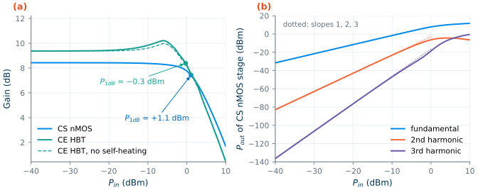
Figure 4.6 shows the result. The CS stage keeps its gain within 0.1 dB up to −7.4 dBm and compresses by 1 dB at IP1dB = +1.1 dBm (OP1dB = +8.5 dBm). The HBT stage behaves differently: its gain rises by 0.85 dB, up to an input of −6 dBm, before it falls, and it passes 1 dB below its small-signal gain at −0.3 dBm. The harmonics of the CS stage follow slopes 2 and 3 at low power; at −20 dBm they are at −31.4 dBc and −64.8 dBc.
To compare with Eqs. (4.15)–(4.16) we need the coefficients \(\alpha_k\). A DC sweep in ngspice gives them: the input is driven through the 25 Ω Thevenin resistance of \(R_S \parallel R_P\), the drain or collector sees the 40 Ω of \(R_D \parallel R_L\) from a supply raised to keep the bias point, and a seventh-order polynomial fitted over ±40 mV gives \(\alpha_1\), \(\alpha_2\) and \(\alpha_3\) of the output voltage against the Thevenin voltage \(V_s/2\). For the CS stage, \(\alpha_1\) = −2.71, \(\alpha_2\) = −5.22 V−1 and \(\alpha_3\) = 3.77 V−2: \(\alpha_3\) opposes \(\alpha_1\), the stage compresses, and Eq. (4.16) predicts an IP1dB of +0.4 dBm, 0.7 dB below harmonic balance. Eq. (4.15) predicts the second harmonic at −20 dBm within 0.9 dB (−30.5 dBc), but puts the third 4.8 dB too low (−69.6 dBc): at 7.3 GHz the transistor’s capacitances add their own distortion. For the HBT stage (isothermal, at its self-heated junction temperature) \(\alpha_3\) = −2.55 V−2 has the same sign as \(\alpha_1\) = −2.96: the exponential characteristic of the bipolar transistor expands, which is why its gain rises before the collector swing clips it. (Self-heating adds to the expansion: the dashed curve, with the HBT’s thermal network switched off at the same junction temperature, rises by 0.60 dB.)
4.6 Intermodulation and intercept points
Harmonics can be filtered; intermodulation often cannot. Apply two tones, \(x = A\cos\omega_1t + A\cos\omega_2t\), and the cube term of Eq. (4.14) produces, among others, components at \(2\omega_1 - \omega_2\) and \(2\omega_2 - \omega_1\) with amplitude \(\tfrac{3}{4}\alpha_3A^3\). If \(\omega_1\) and \(\omega_2\) are two interferers close to the band, spaced by \(\Delta\omega\), these third-order intermodulation (IM3) products fall \(\Delta\omega\) below and above them, possibly right on the wanted channel: two strong Bluetooth or Wi-Fi signals 2 and 4 MHz away from a weak wanted channel put an IM3 product on top of it. The fundamental grows with slope 1 and IM3 with slope 3; extrapolated, the two lines meet at the third-order intercept point, where \(\vert\alpha_1\vert A = \tfrac{3}{4}\vert\alpha_3\vert A^3\):
Key equation · Third-order intercept point
\[A_{IIP3} = \sqrt{\frac{4}{3}\left\vert\frac{\alpha_1}{\alpha_3}\right\vert}, \qquad \frac{A_{1dB}^2}{A_{IIP3}^2} = \frac{0.145}{4/3} = 0.109\ \ (-9.6\ \mathrm{dB}). \tag{4.17–4.18}\]The input power at the intercept is the IIP3, the output power the OIP3 = IIP3 + gain. For a compressive third-order nonlinearity, IP1dB lies 9.6 dB below IIP3.
The intercept is never reached: the stage compresses long before. It is found by extrapolation from a measurement at low power, where both lines have their ideal slopes. If the IM3 products are \(\Delta P_3\) decibels below the fundamental at an input power \(P_{in}\) per tone, then
\[\mathrm{IIP3} = P_{in} + \frac{\Delta P_3}{2}, \qquad \mathrm{IIP2} = P_{in} + \Delta P_2. \tag{4.19}\]The square term produces second-order intermodulation (IM2) at \(\omega_1 \pm \omega_2\) with amplitude \(\alpha_2A^2\), growing with slope 2. Its intercept is
\[A_{IIP2} = \left\vert\frac{\alpha_1}{\alpha_2}\right\vert. \tag{4.20}\]In a narrowband heterodyne receiver IM2 falls out of band, but in a zero-IF or low-IF receiver the difference frequency \(\omega_2 - \omega_1\) of two interferers, or the envelope of one amplitude-modulated interferer, lands at baseband next to the wanted signal, which is why IIP2 is a key specification of direct-conversion receivers [68] (Chapter 5).
We applied two tones at 2.440 and 2.441 GHz with Xyce (seven harmonics of each and intermodulation products up to seventh order, 113 frequencies), sweeping the power per tone:
* two-tone harmonic-balance sweep of the CS stage (Xyce; the script adds the model library)
.param amp=0.01
vdd  vdd 0 1.2
vs0  s0 0  sin(0 {amp} 2.44e9)          ; tone 1, peak amplitude amp
vs1  s1 s0 sin(0 {amp} 2.441e9)         ; tone 2, in series
rs   s1 in 50
cin1 in g1 100p
rp1  g1 b1 50
vb1  b1 0 0.65
XM1  d1 g1 0 0 sg13_lv_nmos W=50u L=0.13u ng=10 m=4
lc1  vdd d1 1u
rd1  vdd d1 200
co1  d1 out 100p
rl   out 0 50
.hb 2.44e9 2.441e9
.options hbint numfreq=7,7 intmodmax=7 startupperiods=2
.step amp list 6.32456e-03 7.96214e-03 ...    ; P_in = amp^2/(8*50)
.print hb_fd v(out) v(g1) v(s0)
Figure 4.7a shows the output spectrum of the CS stage at −20 dBm per tone: the two tones, the IM3 pair 1 MHz outside them, and fifth-order products 2 MHz out. Figure 4.7b shows the sweeps. Below −26 dBm the fitted slopes are 1.00 and 3.00 for the CS stage, 1.00 and 3.00 for the CE stage. The extrapolated intercepts are IIP3 = +11.2 dBm for the CS stage and +2.1 dBm for the CE stage, and from the sum frequency \(f_1 + f_2\), IIP2 = +5.3 and −7.9 dBm. (We read IM2 at \(f_1 + f_2\) because the choke shorts the 1 MHz difference product at the output; for a memoryless stage both have the amplitude \(\alpha_2A^2\).)
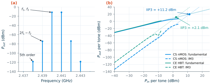
The CS stage is the more linear one by 9.1 dB, at three times the current. Its IIP3 lies 10.1 dB above its IP1dB, close to the classic 9.6 dB of Eq. (4.18). The HBT stage breaks the rule: its IIP3 is only 2.4 dB above the point where its gain has fallen 1 dB below the small-signal value. Its expansion delays compression, while IM3 grows from the start. The 9.6 dB rule assumes a compressive third-order term that dominates all the way to compression; use it as a first guess, never instead of a two-tone simulation.
How well do the Taylor coefficients predict the intercepts? For the CS stage, Eq. (4.17) gives +10.0 dBm against +11.2 dBm, and Eq. (4.20) +4.5 dBm against +5.3 dBm: the power series of the DC characteristic describes the MOSFET stage to about a decibel. For the HBT stage, IIP2 agrees (−8.0 against −7.9 dBm), but IIP3 does not: the isothermal coefficients predict +11.9 dBm, 9.8 dB more than harmonic balance. Three effects that a DC sweep cannot see are responsible, and harmonic balance can switch them off one at a time:
- Self-heating. The HBT runs 6.5 K above ambient, and with a thermal time constant of 5.4 ns its junction temperature follows the power envelope of the two tones, which beats at 1 MHz. The temperature swing modulates the gain and adds IM3. Without the thermal network, at the same junction temperature, the IIP3 rises by 5.6 dB to +7.7 dBm, and its distance from IP1dB grows to 8.2 dB.
- Nonlinear charge. The diffusion capacitance of the base-emitter junction grows exponentially with \(V_{BE}\), like the current. A DC sweep ignores it, but at gigahertz frequencies its nonlinear charging current adds distortion of its own. The third harmonic shows it plainly: −56.1 dBc at −20 dBm, against the −73.4 dBc that \(\alpha_3\) predicts.
- Out-of-band terminations. The second-order products at DC, \(f_2 - f_1\) and \(2f\) mix with the tones again and add to IM3, and the impedances they see differ from the signal’s: the choke shorts the output at low frequencies, and the blocking capacitor leaves the input on \(R_P\) alone. With frequency-independent terminations (a DC-coupled source, and the 40 Ω load at DC too), the HBT’s isothermal IIP3 hardly moves, to +7.5 dBm, but the CS stage’s falls by 2.1 dB to +9.1 dBm.
A power series describes a memoryless stage. When charges, temperatures or even-order products with their own impedances matter, a Volterra-series analysis [17] or a harmonic-balance simulation of the complete circuit is needed.
What this means for your design
Linearity is a property of the complete circuit, not of the transistor’s DC curve. Bias networks, chokes and decoupling set the impedances that even-order products see; the thermal time constant of a bipolar transistor makes its IM3 depend on the spacing of the tones. Simulate two tones in harmonic balance with the real bias network and with tone spacings like those of the real interferers.
4.7 Blocking, desensitization and cross-modulation
A weak wanted signal often arrives together with a strong unwanted one, a blocker: a nearby phone, a Wi-Fi access point, or, for a 2.4 GHz receiver, an LTE band 40 transmitter at 2.3–2.4 GHz. With the wanted signal \(A_1\cos\omega_1t\) much smaller than the blocker \(A_B\cos\omega_Bt\), the cube term of Eq. (4.14) gives the wanted signal a gain
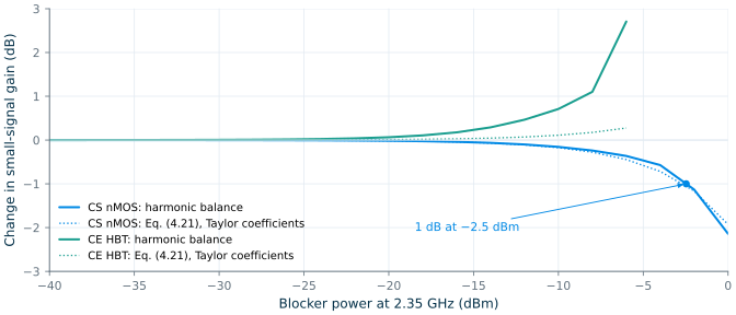
\[\alpha_{1,eff} = \alpha_1 + \frac{3}{2}\alpha_3A_B^2, \tag{4.21}\]twice the \(A^2\) term of the single-tone compression. A compressive stage loses small-signal gain, and with it sensitivity: desensitization. The wanted gain falls by 1 dB at \(A_B^2 = 0.0726\,\vert\alpha_1/\alpha_3\vert\), half the \(A_{1dB}^2\) of Eq. (4.16): a blocker desensitizes by 1 dB at about 3 dB below the stage’s own IP1dB. If the blocker is amplitude modulated, \(A_B(1 + m\cos\omega_mt)\), the gain of Eq. (4.21) varies with the modulation, and the wanted signal acquires an amplitude modulation of index about \(3(\alpha_3/\alpha_1)A_B^2m\): cross-modulation [6, 67],
\[y_{\omega_1} \approx \left[\alpha_1 + \frac{3}{2}\alpha_3A_B^2\left(1 + 2m\cos\omega_mt\right)\right]A_1\cos\omega_1t. \tag{4.22}\]Figure 4.8 shows desensitization in harmonic balance: a −50 dBm wanted tone at 2.44 GHz and a blocker at 2.35 GHz swept from −40 to 0 dBm. The CS stage loses 1 dB of gain at a blocker power of −2.5 dBm, 3.6 dB below its IP1dB, close to the 3 dB of the third-order model; the dotted line, Eq. (4.21) with the Taylor coefficients, follows the simulation up to 0 dBm. The HBT stage’s wanted gain instead rises, by 2.71 dB at a −6 dBm blocker (beyond which harmonic balance did not converge), ten times the 0.27 dB that its small positive \(\alpha_3\) predicts. The blocker raises the average collector current, by rectification in the exponential characteristic and by heating the junction, and the transconductance rises with it: a bias shift that the cubic term alone does not capture. Neither direction is good news: a gain that depends on the blocker also turns the blocker’s amplitude modulation into cross-modulation.
A receiver meets its blocking specification with filtering before the first nonlinear stage, and with enough headroom in the LNA and mixer for whatever the filter lets through. Two other effects of a blocker are covered later: reciprocal mixing, the blocker mixing with the phase noise of the LO (Chapter 11), and the IM2 of a modulated blocker in a low-IF receiver (Chapter 10).
Table 4.1 collects the results for the two test stages.
Table 4.1. The two test stages of this chapter (2.44 GHz, tt, 27 °C; noise from ngspice with the RF MOSFET model, linearity from Xyce harmonic balance; Taylor: from the coefficients of the DC transfer characteristic).
| CS nMOS stage | CE HBT stage | |
|---|---|---|
| Transistor, supply current | 4 × 50/0.13 µm, 9.81 mA | npn13G2 Nx = 8, 3.06 mA |
| gm, equivalent noise resistance Rn | 74.6 mS, 25.1 Ω | 74.3 mS, 26.1 Ω |
| \(\vert S_{21}\vert^2\), \(S_{11}\) | 8.22 dB, −15.1 dB | 9.38 dB, −27.3 dB |
| NF: simulated / Eq. (4.9) | 6.22 / 6.22 dB | 6.33 / 6.31 dB |
| IP1dB: harmonic balance / Taylor | +1.1 / +0.4 dBm | −0.3 dBm / — (expansive) |
| IIP3: harmonic balance / Taylor | +11.2 / +10.0 dBm | +2.1 / +11.9 dBm |
| IIP3 − IP1dB | 10.1 dB | 2.4 dB |
| IIP2: harmonic balance / Taylor | +5.3 / +4.5 dBm | −7.9 / −8.0 dBm |
| Blocker at 2.35 GHz: 1 dB desensitization / gain change at −6 dBm | −2.5 dBm / −0.36 dB | none / +2.71 dB |
4.8 Cascaded linearity and dynamic range
In a cascade, each stage’s distortion adds to that of the stages before it. Take two memoryless stages with coefficients \(\alpha_k, \beta_k\). The IM3 at the output has two parts: the first stage’s IM3, \(\tfrac{3}{4}\alpha_3A^3\), amplified by \(\beta_1\), and the second stage’s IM3 of the amplified tones, \(\tfrac{3}{4}\beta_3(\alpha_1A)^3\). If they add in phase, the worst case, the input intercept of the cascade follows from adding the inverse squares of the intercepts referred to the input [6]:
Key equation · Cascaded IIP3
\[\frac{1}{A_{IIP3}^2} = \frac{1}{A_{IIP3,1}^2} + \frac{\alpha_1^2}{A_{IIP3,2}^2} + \frac{\alpha_1^2\beta_1^2}{A_{IIP3,3}^2} + \dots \tag{4.23}\]or, with powers in watts and available power gains \(G_k\) (matched stages),
\[\frac{1}{\mathrm{IIP3}} = \frac{1}{\mathrm{IIP3}_1} + \frac{G_1}{\mathrm{IIP3}_2} + \frac{G_1G_2}{\mathrm{IIP3}_3} + \dots \tag{4.24}\]
Eq. (4.24) mirrors the Friis formula: in a cascade the first stages set the noise and the last stages set the distortion, and the gain in front of a stage helps the one and hurts the other (Figure 4.4). Our two CS stages in series are a test: each has an IIP3 of +11.2 dBm and a gain of 8.43 dB, so Eq. (4.24) predicts +2.2 dBm, dominated by the second stage, whose intercept referred to the input is +2.8 dBm. A two-tone simulation of the cascade gives +0.4 dBm, 1.8 dB worse. Eq. (4.23) keeps only the third-order terms of each stage. In our broadband cascade the first stage’s second harmonic and sum-frequency products reach the second stage and mix with the tones in its \(\alpha_2\), adding a term \(2\alpha_1\alpha_2\beta_2\) to the cascade’s cubic coefficient. In a narrowband receiver, tuned loads and filters between the stages remove these products, and Eq. (4.24) applies.
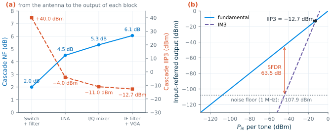
The noise floor and the intercept together set the dynamic range. Referred to the input, the noise floor in the bandwidth \(B\) is \(P_{floor} = -174 + 10\log_{10}B + \mathrm{NF}\) (dBm). Raise two tones until their IM3 products reach this floor: the tones are then as far above the floor as the system can go without its own distortion showing, the spurious-free dynamic range. Since IM3 rises three times as fast as the tones, from Eq. (4.19),
\[\mathrm{SFDR} = \frac{2}{3}\left(\mathrm{IIP3} - P_{floor}\right). \tag{4.25}\]Table 4.2 puts the pieces together for the course receiver. The block numbers are illustrative targets for the designs of Chapters 9 and 10; Chapter 19 replaces them with the designed blocks.
Table 4.2. Cascade budget of the course receiver with illustrative block numbers. "Cascade" columns: from the antenna to the output of the block, with Eqs. (4.11) and (4.24).
| Block | Gain (dB) | NF (dB) | IIP3 (dBm) | Cascade gain (dB) | Cascade NF (dB) | Cascade IIP3 (dBm) |
|---|---|---|---|---|---|---|
| Switch + filter | −2 | 2 | +40 | −2 | 2.00 | +40.0 |
| LNA | +16 | 2.5 | −6 | +14 | 4.50 | −4.0 |
| I/Q mixer | +8 | 12 | +4 | +22 | 5.33 | −11.0 |
| IF filter + VGA | +30 | 20 | +14 | +52 | 6.06 | −12.7 |
The receiver has an NF of 6.06 dB and an IIP3 of −12.7 dBm, inside the course targets of 8 dB and −15 dBm; the front end up to the mixer alone has −11.0 dBm. With the 12.3 dB SNR of Section 4.4, the sensitivity is −95.6 dBm, and with a noise floor of −107.9 dBm in 1 MHz the SFDR is 63.5 dB (Figure 4.9). The two budgets pull in opposite directions. The switch and filter (whose loss enters the NF in full) and the LNA account for 39 % and 31 % of the excess noise factor, while the mixer and the IF stage, behind 14 and 22 dB of gain, contribute 53 % and 34 % of the distortion. More LNA gain would lower the NF and the IIP3 together; without the 2 dB filter loss, the NF would be 4.06 dB.
Try it · The noise and linearity script
Every number in this chapter comes from
tools/figs/ch04_noise_linearity.py:python3 tools/figs/ch04_noise_linearity.py devnoise friis sens hb desense budget(add--resimto rerun the harmonic-balance simulations, about half an hour). Three experiments: (1) changeRDfrom 200 to 1000 Ω and rerunfriis: by Eq. (4.9) the \(R_D\) term shrinks, but what happens to the gain and to the Friis error of the CS → CS cascade? (2) SetF2to 2.54 GHz, a tone spacing of 100 MHz, well above the HBT’s thermal corner of about 30 MHz, and rerunhb --resim: does the HBT’s IIP3 move towards the +7.7 dBm it has without self-heating? (3) InBLOCKS, raise the LNA gain to 20 dB and rerunbudget: by how much do the NF and the IIP3 of the receiver move, and which way?
- Thermal noise, \(4kTR\), and shot noise, \(2qI\), are white; flicker noise rises as 1/f below a corner of 11.5 MHz in the course nMOS and 239 Hz in its HBT. At radio frequencies a transistor’s noise is an equivalent noise resistance Rn: about 25 Ω for both devices at 74.5 mS.
- The noise figure, defined with a 290 K source, counts the noise a block adds. A resistively terminated stage cannot beat 3 dB; ours reach 6.22 dB (CS) and 6.33 dB (CE), as Eq. (4.9) predicts. ngspice references its NF to the circuit temperature: correct it.
- The Friis formula is exact when it uses available gains and each stage’s NF for the source impedance it sees; a loss in front of the LNA adds to the NF decibel for decibel.
- Sensitivity is −174 dBm/Hz + 10 log B + NF + SNRmin. GFSK with a discriminator needs 12.3 dB for 0.1 % BER, so the course’s −90 dBm allows an NF of 11.7 dB; the 8 dB specification keeps 3.7 dB of margin.
- A power series predicts harmonics, compression, IM3, IM2 and desensitization, and the 9.6 dB gap between IP1dB and IIP3, for a compressive, memoryless stage: the CS stage follows it to about a decibel (IIP3 +11.2 dBm, gap 10.1 dB). The HBT stage, which expands, heats up and has nonlinear charge, shows where that picture ends (IIP3 +2.1 dBm, gap 2.4 dB): simulate two tones in harmonic balance.
- In a cascade the first stages set the noise figure and the last stages the intercept; the illustrative course receiver reaches NF 6.06 dB, IIP3 −12.7 dBm and a spurious-free dynamic range of 63.5 dB in 1 MHz.
Further reading
- B. Razavi, RF Microelectronics [6], Chapter 2: noise figure, sensitivity, nonlinearity, intercept points and dynamic range, at the level of this chapter and with many more examples.
- T. H. Lee, The Design of CMOS Radio-Frequency Integrated Circuits [7], Chapters 11–12: the physics of noise in resistors and transistors, and the noise of two-ports.
- H. T. Friis, “Noise figures of radio receivers” [62], the short paper that defined the noise figure and the cascade formula; H. Rothe and W. Dahlke [63] for the noise parameters of a two-port.
- S. A. Maas, Nonlinear Microwave and RF Circuits [16], and P. Wambacq and W. Sansen, Distortion Analysis of Analog Integrated Circuits [17]: harmonic balance, Volterra series and why real circuits depart from a power series.
- K. S. Kundert, “Introduction to RF simulation and its application” [32]: harmonic balance and the other steady-state methods behind the simulations of this chapter.