Lab 0
Tools and a First S-Parameter
Start the container, get the course files, and follow one S-parameter simulation from the netlist to a Touchstone file and into scikit-rf: |S| in decibels, a Smith chart and an impedance.
- Install IIC-OSIC-TOOLS 2026.10 and run a lab both inside the container and from your own computer.
- Run an ngspice
spanalysis with noise, and write its results as a Touchstone file and a noise-parameter table.- Read a Touchstone file by eye and with scikit-rf, and turn it into gains, impedances, stability factors and noise parameters.
- Check a simulator’s noise figure against the noise-parameter formula by hand.
Contents
| Lab 0 at a glance | |
|---|---|
| Goal | A working container, the course files, and the S-parameters of Chapter 2’s amplifier read three ways with scikit-rf. |
| Chapters | Chapter 1 (Section 1.5, Figure 1.6) and Chapter 2 (Sections 2.1–2.3 and 2.8) |
| Time | 1–2 hours, most of it downloading the image |
| Files | tools/labs/lab0/: amp_sp.cir, lab0.py; tools/labs/common/: labkit.py, iic.sh |
| Run time | amp_sp.cir under a second; lab0.py about 3 s; Chapter 1’s script about 1 min |
Hand calculation
The circuit is the 2.44 GHz common-emitter amplifier of Figure 2.1: one npn13G2 with four emitter fingers at \(I_C\) = 2.00 mA, an RF choke \(L_C\) = 100 nH in parallel with \(R_C\) = 150 Ω, two L-sections and two 10 pF DC blocks. Before you simulate:
- Choke and DC blocks. Compute the reactance of \(L_C\) and of one DC block at 2.44 GHz. Compared with \(R_C\) and with 50 Ω, which of them can you ignore?
-
Noise figure from noise parameters. Chapter 2 reports \(NF_{min}\) = 2.02 dB, \(R_n\) = 53.6 Ω and \(\Gamma_{opt}\) = 0.644∠−22.7° at 2.44 GHz. With a 50 Ω source (\(\Gamma_s\) = 0), Eq. (6.11) of Chapter 6 reduces to
\[F = F_{min} + \frac{4R_n}{Z_0}\,\frac{\vert\Gamma_{opt}\vert^2}{\vert 1 + \Gamma_{opt}\vert^2}.\]Compute \(F\) and \(NF = 10\log_{10}F\). This is the check that tells you that ngspice’s
nfminis in decibels,rnin ohms andsopta reflection coefficient. - What “matched” means. If \(\vert S_{11}\vert\) = −53 dB, how far can the input impedance be from 50 Ω? And if both ports are matched, how do the transducer gain \(\vert S_{21}\vert^2\) and the maximum available gain compare?
Steps
-
Install Docker and IIC-OSIC-TOOLS. Follow the README of IIC-OSIC-TOOLS [193] (Section 2.2 of The Art of Analog IC Design walks through it): install Docker Desktop (macOS, Windows) or Docker Engine (Linux), then
git clone --depth=1 https://github.com/iic-jku/iic-osic-tools.git cd iic-osic-tools DOCKER_TAG=2026.10 ./start_vnc.sh # desktop in your browser: http://localhost/?password=abc123DOCKER_TAGpins the release the course was simulated with; the image is several gigabytes, so keep 20 GB of disk free. The start script mounts~/eda/designsof your computer as/foss/designsin the container: keep all your work there. If you will only work from your own terminal,docker pull hpretl/iic-osic-tools:2026.10is enough. -
Put the course files in place. Copy the
rfic-designfolder of course files into~/eda/designson your computer, which is/foss/designsin the container. In a terminal of the container’s desktop:cd /foss/designs/rfic-design/tools/labs/lab0 && ls # amp_sp.cir lab0.py lab_numbers.jsonFrom your own computer, every command below runs through the container with
../common/iic.sh; try it now (the first call takes a few seconds to start the container):cd ~/eda/designs/rfic-design/tools/labs/lab0 ../common/iic.sh ngspice -v # ngspice-47 -
Simulate. Open
amp_sp.cirin an editor. It is Chapter 2’s netlist with two additions after thespanalysis:wrs2pwrites the S-parameters as a Touchstone 1.0 file andwrdatawrites the noise parameters, one row per frequency. Run it:ngspice -b amp_sp.cir # from your computer: ../common/iic.sh ngspice -b amp_sp.cirIt prints the collector current and, at 2.44 GHz, \(\vert S_{21}\vert\), \(\vert S_{11}\vert\), the noise figure and \(NF_{min}\), and writes
out/amp.s2pandout/amp_noise.txt. -
Read the Touchstone file by eye.
head -7 out/amp.s2pshows the option line# Hz S RI R 50(frequency in hertz, S-parameters, real and imaginary parts, 50 Ω) and one line per frequency with S11, S21, S12, S22 (Appendix B, Section B.5). Find the 2.44 GHz line and check that S21 has a magnitude of about 8.3. -
Read it with scikit-rf. Start
python3in the same folder (from your computer:../common/iic.sh python3) and type:import skrf as rf amp = rf.Network("out/amp.s2p") print(amp) # 2-Port Network: 0.5-4 GHz, 351 points, z0 = 50 ohm a = amp["2.44GHz"] # one frequency a.s_db # |S11| |S12| / |S21| |S22| in dB a.s11.z # the input impedance with port 2 terminated in 50 ohm amp.stability[amp.f == 2.44e9] # Rollett's KA
Networkholds S, and computes Y, Z, ABCD, gains and stability from it on request. -
Three views of the same file. Run the lab script:
python3 lab0.py # from your computer: ../common/iic.sh python3 lab0.pyIt reruns the netlist, reads both files with
labkit.read_sp(which attaches the noise parameters to theNetwork, so thatamp.nfmin_db,amp.g_opt,amp.z_optandamp.rnwork), prints the checkpoint numbers and draws Figure L0.1 intoout/lab0_amp.png. μ is not part of scikit-rf; the script computes it from its definition in Chapter 3 in two lines. -
A chapter script. Every figure and number of the chapters comes from a script in
tools/figs/. Run Chapter 1’s transistor simulation from the top of the course files:cd /foss/designs/rfic-design python3 tools/figs/ch01_why_rf.py gain # about a minute; writes tools/figs/ch01_numbers.jsonIt simulates an SG13G2 nMOS, an
npn13G2and a SKY130 nMOS and redraws Figure 1.6 asassets/figs/ch01_gain.svgin the course folder. Look upgmax_2g44_dBandgmax_50g_dBin the JSON file.
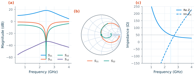
sp, read with scikit-rf. (a) |Sij| in dB; shaded: 2.400–2.4835 GHz. (b) S11 and S22 on the Smith chart (open circles: 0.5 GHz; dots: 2.44 GHz). (c) Input impedance with port 2 terminated in 50 Ω.Checkpoint
Table L0.1. Lab 0 results (typical models, 27 °C, at 2.44 GHz unless stated). Tolerance: ±1 in the last digit shown, except where stated.
| Quantity | Lab 0 | Chapter |
|---|---|---|
| Hand calculation: reactance of \(L_C\) / of one DC block | 1.53 kΩ / 6.52 Ω | |
| Hand calculation: NF from the noise parameters (±0.01 dB) | 3.57 dB | 3.569 dB (Ch. 2) |
| Collector current | 2.001 mA | 2.00 mA (Ch. 2) |
| \(\vert S_{21}\vert\) / \(\vert S_{11}\vert\) / \(\vert S_{22}\vert\) / \(\vert S_{12}\vert\) | 18.35 / −53.0 / −62.8 / −33.6 dB | 18.35 / −53.0 / −62.8 / −33.6 dB (Ch. 2) |
| In the band 2.400–2.4835 GHz: \(\vert S_{21}\vert\); worst \(\vert S_{11}\vert\), \(\vert S_{22}\vert\) | 18.33–18.35 dB; −22.4, −29.3 dB | 18.33 dB at both edges; −22.4, −29.3 dB (Ch. 2) |
| Input impedance \(Z_{in}\) (port 2 in 50 Ω) | 49.9 − j0.2 Ω | |
| Rollett \(K\), \(\mu\) | 2.99, 5.79 | 2.99, 5.79 (Ch. 2) |
Maximum available gain (max_gain) |
18.35 dB | |
| NF, \(NF_{min}\) | 3.57, 2.02 dB | 3.57, 2.02 dB (Ch. 2) |
| \(R_n\), \(\Gamma_{opt}\), \(Z_{opt}\) | 53.6 Ω, 0.644∠−22.7°, 129.2 − j109.6 Ω | 53.6 Ω, 0.644∠−22.7° (Ch. 2) |
| Chapter 1’s script: Gmax of the SG13G2 nMOS / npn13G2 at 2.44 GHz | 20.0 / 29.0 dB | |
| Chapter 1’s script: Gmax at 50 GHz | 3.56 / 15.8 dB | 3.6 / 15.8 dB (Ch. 1) |
Every simulated row reproduces Chapter 2. The hand calculation of step 2 gives \(F\) = 1.592 + 4 × 1.072 × 0.4147/2.603 = 2.275, so NF = 3.57 dB, the value ngspice reports. ch01_numbers.json from step 7 must equal the file that came with the course files, all 99 numbers of the gain part.
Questions
- The maximum available gain equals \(\vert S_{21}\vert^2\) at 2.44 GHz to the second decimal. Why must it, for an amplifier whose two ports are both conjugately matched? Away from 2.44 GHz, which is larger, and why?
- \(NF\) = 3.57 dB is 1.55 dB above \(NF_{min}\). The input L-section was designed for a power match, not a noise match. Where on the Smith chart would the source have to be for \(NF_{min}\), and what would that do to \(\vert S_{11}\vert\)?
- In Figure L0.1c the input impedance is 50 Ω only near 2.44 GHz. Which elements of the circuit set how fast it moves away, and how does that show in panel (a)?
wrs2pneeds a vector calledRbase. What would go wrong if the ports had different reference impedances, and how would you then describe the file to scikit-rf?
Extension
Change \(R_C\) from 150 Ω to 300 Ω in amp_sp.cir and rerun lab0.py. The match is now wrong: read the new \(Z_{in}\) and output impedance, \(K\) and the maximum available gain from the printout, and compare \(\vert S_{21}\vert^2\) with the maximum available gain. Then redesign the output L-section for the new collector resistance with Eq. (8.3) of Chapter 8 (the series element must also absorb the 6.52 Ω of the DC block) and see how close your values bring \(\vert S_{22}\vert\) to Chapter 2’s −62.8 dB. Why is the hand design not exact? (Hint: the transistor’s \(C_\mu\) couples the output network to the input.)