Chapter 2
Simulating RF Circuits
An RF designer asks questions that plain SPICE was not built to answer: what are the S-parameters and the noise figure at 2.44 GHz, where does the gain compress, how strong are the intermodulation products of two channels 2 MHz apart? This chapter takes one small amplifier through every analysis the open-source tools offer, from the operating point to harmonic balance and an electromagnetic solver, shows where they agree and where they mislead, and ends with a table that says which analysis answers which question.
- Set up ports, sources and loads so that ngspice and Xyce report the S-parameters, noise figure, gain, compression and intermodulation of an RF circuit.
- Run operating-point, AC, noise and S-parameter analyses in ngspice, and relate their results to each other.
- Run transient simulations whose spectra can be trusted: choose the time step, wait for the steady state, and use coherent sampling or a window.
- Explain harmonic balance, and use Xyce’s
.HBfor single-tone compression and two-tone intermodulation.- Explain the difference between FDTD (openEMS) and FEM (Palace) electromagnetic solvers, run an IHP openEMS example, and choose the right analysis for a question.
Contents
- 2.1 Why SPICE alone is not enough
- 2.2 Operating point, AC and noise analysis
- 2.3 S-parameter analysis in ngspice
- 2.4 Transient analysis of RF circuits
- 2.5 Harmonic balance in Xyce
- 2.6 Periodic steady state and transient noise
- 2.7 Electromagnetic simulation with openEMS and Palace
- 2.8 Post-processing in Python
- 2.9 Choosing the right analysis
- Further reading
2.1 Why SPICE alone is not enough
SPICE was written to find the DC operating point, the small-signal AC response and the transient response of a circuit. An RF circuit stretches each of these. First, the quantities RF designers specify are defined in a steady state: the S-parameters and noise figure of Chapters 3 and 4, referred to 50 Ω ports, and the compression, harmonics and intermodulation of a circuit driven by one or two sinusoids for ever. A transient simulation reaches that state only after the start-up has died out. Second, the time scales spread over orders of magnitude: a 2.44 GHz period is 410 ps, a bias network settles in tens of nanoseconds, and two Bluetooth channels 2 MHz apart beat with a period of 500 ns. A transient that resolves picoseconds over microseconds is slow. Third, at gigahertz frequencies the interconnect and the passives are circuits in their own right, and only an electromagnetic (EM) solver can tell what they do. Kundert’s tutorial [32] surveys the methods that grew out of these needs.
The open-source answer is a set of tools, all in IIC-OSIC-TOOLS [193]: ngspice [194] for the operating point, AC, noise, S-parameter and transient analyses; Xyce [195] for harmonic balance and multi-time methods; openEMS [196] and Palace [197] for the EM simulation of layouts; and Python to glue them together. This chapter uses all of them on one circuit.
The running example
Figure 2.1 shows it: a common-emitter amplifier for the course radio’s 2.4 GHz band, built around one SG13G2 SiGe HBT, npn13G2 with four emitter fingers (\(N_x\) = 4), biased at \(I_C\) = 2.00 mA from the 1.2 V supply. A 1 kΩ resistor \(R_B\) from \(V_{BB}\) = 0.845 V sets the base voltage (\(V_{BE}\) = 0.842 V, \(I_B\) = 2.79 µA, so \(\beta\) = 718); the stage draws 2.4 mW. The collector is fed through an RF choke \(L_C\), an inductor large enough (100 nH, 1.5 kΩ at 2.44 GHz) to carry the DC current without loading the signal. The resistor \(R_C\) = 150 Ω in parallel with it sets the output resistance and keeps the stage stable: on its own, the stage has a Rollett factor \(K\) = 2.99 at 2.44 GHz (Chapter 3). DC blocks \(C_{B1}\) and \(C_{B2}\) keep the bias off the 50 Ω ports.
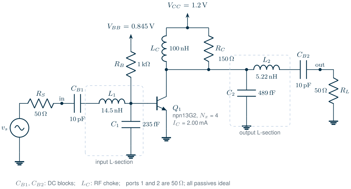
The bare stage is far from 50 Ω: its input impedance at 2.44 GHz is 704 − j402 Ω and its output impedance 150 + j5 Ω. Two L-sections, each a series inductor and a shunt capacitor, transform both to 50 Ω. The figure script computes them for a simultaneous conjugate match at 2.44 GHz, with the DC blocks counted as part of the series branch, and rounds them to three digits; Chapter 8 explains the method. Every passive is ideal; Chapter 7 makes them real. The stage is a vehicle for the simulators, not a finished design: Chapter 9 designs the course LNA properly.
2.2 Operating point, AC and noise analysis
ngspice describes a port as a voltage source with two extra parameters: portnum, its number, and z0, its reference impedance, which the source also uses as its internal resistance. In an .ac or .noise analysis a port behaves as an AC source of the given amplitude behind 50 Ω, or, with ac 0, as a 50 Ω termination; in an .sp analysis it defines where the S-parameters are measured. One netlist therefore serves all the small-signal analyses. The listing is the complete deck, as it runs in IIC-OSIC-TOOLS with ngspice -b ch02_amp.cir:
* Chapter 2 running example: 2.44 GHz common-emitter amplifier, IHP SG13G2 npn13G2
.lib /foss/pdks/ihp-sg13g2/libs.tech/ngspice/models/cornerHBT.lib hbt_typ
VCC   vcc  0    1.2
VBB   bb   0    0.845
RB    bb   b    1k
XQ1   c    b    0 0 npn13G2 Nx=4
LC    vcc  c    100n
RC    vcc  c    150
CB1   in   m1   10p
L1    m1   b    14.5n
C1    b    0    235f
C2    c    0    489f
L2    c    m2   5.22n
CB2   m2   out  10p
V1    in   0    dc 0 ac 1 portnum 1 z0 50
V2    out  0    dc 0 ac 0 portnum 2 z0 50
.control
op
print i(vcc) v(b) i(vbb)
ac dec 50 100meg 10g
noise v(out) v1 lin 1 2.44g 2.44g 1
print inoise_spectrum onoise_spectrum
sp lin 3 2.4g 2.48g 1
print s_1_1 s_2_1 nf nfmin rn sopt
.endc
.end
The operating point (op) comes first, because every small-signal analysis linearizes the circuit around it: \(I_C\) = 2.001 mA and \(V_{BE}\) = 0.842 V, as designed.
The AC analysis (ac) then gives the node voltages for a 1 V source. With a source of EMF \(v_s\) behind \(Z_0\) and a load \(Z_0\), the wave incident on port 1 is \(v_s/2\) and the wave leaving port 2 is \(v_{out}\), so
At 2.44 GHz, \(\vert v_{out}\vert\) = 4.137 V, so \(\vert S_{21}\vert\) = 18.355 dB, exactly what the S-parameter analysis of Section 2.3 reports. The matched input sees 0.5 V, and the input L-section steps it up 4.44 times at the base: a lossless match is a resonant transformer.
The noise analysis (noise v(out) v1 ...) computes the noise spectral density at the output, onoise_spectrum, and refers it to the input source through the gain, inoise_spectrum. With a last argument (points per summary, here 1) it also stores the contribution of every noise source. Here is the first trap: the internal resistance of an ngspice port is noiseless in .noise, so inoise_spectrum holds only the noise the amplifier adds. The noise factor is then
with \(R_S\) = 50 Ω and \(T\) the simulation temperature. The simulated \(\overline{v_{n,in}^2}^{1/2}\) = 1.028 nV/√Hz gives NF = 10 log F = 3.569 dB at 2.44 GHz, equal to the .sp result to the third decimal. Table 2.1 splits the output noise into its sources.
Table 2.1. Where the output noise of the amplifier comes from at 2.44 GHz (ngspice `.noise` with a summary; the source's own share computed from the `.ac` gain).
| Source | Share of the output noise |
|---|---|
| 50 Ω source | 44.0 % |
| Bias resistor \(R_B\) (1 kΩ) | 43.1 % |
| Transistor \(Q_1\), total | 12.2 % |
| — base resistances | 6.3 % |
| — base shot noise | 2.6 % |
| — collector shot noise | 1.9 % |
| — other terms | 1.4 % |
| Collector resistor \(R_C\) | 0.7 % |
What this means for your design
The bias resistor adds almost as much noise as the source itself: the noise current of 1 kΩ at the base is not small next to the signal current from a 704 Ω input. A noise analysis with a summary tells you in one run which element to change. Here a larger \(R_B\) fed from a bias circuit, or an inductive bias feed, would lower the noise figure; Chapter 9 does that and also matches the source for noise rather than for power.
Which temperature?
The IEEE defines the noise figure with the source at \(T_0\) = 290 K [187], but ngspice simulates at 27 °C (300.15 K) and refers the noise figure to the simulation temperature. A matched 6.00 dB resistive attenuator makes the check: .sp reports a noise figure of 6.00 dB at 27 °C and at 16.85 °C (290 K) alike, equal to the loss, while the IEEE value for an attenuator at 27 °C is 6.11 dB. To convert a noise figure \(F_T\) simulated at \(T\),
which turns our 3.57 dB into 3.65 dB. The difference is small, but it is systematic, and it grows with the noise figure.
2.3 S-parameter analysis in ngspice
sp lin 351 0.5g 4g 1 sweeps 351 frequencies and computes the S-, Y- and Z-parameters between all ports (s_1_1, s_2_1, …, y_1_1, …, z_2_2); the final 1 adds a noise analysis that returns the noise figure nf for 50 Ω sources, the four noise parameters nfmin, rn and sopt (\(\Gamma_{opt}\)) and the noise-correlation matrix cy_i_j [39]. nf and nfmin are in dB: recomputing the noise figure from nfmin, rn and sopt with the formula of Chapter 4 gives 3.569 dB, the value of nf.
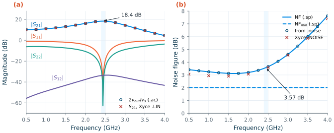
.sp (lines), S21 from .ac with Eq. (2.1) (circles) and from Xyce's .LIN (crosses). (b) Noise figure and minimum noise figure from .sp, noise figure from .noise with Eq. (2.2) (circles) and from Xyce's .NOISE (crosses). Shaded: the 2.4 GHz band. 27 °C, typical models.Figure 2.2 shows the result. At 2.44 GHz the gain is \(\vert S_{21}\vert\) = 18.35 dB, 18.33 dB at both band edges; the match is almost perfect at the design frequency (\(\vert S_{11}\vert\) = −53.0 dB, \(\vert S_{22}\vert\) = −62.8 dB) and better than −22.4 dB and −29.3 dB across the band. The reverse gain \(\vert S_{12}\vert\) is −33.6 dB, and at 2.44 GHz the amplifier is unconditionally stable (\(K\) = 2.99, \(\mu\) = 5.79). The noise figure is 3.57 dB (3.52–3.62 dB across the band) while \(\mathrm{NF}_{min}\) = 2.02 dB, with \(R_n\) = 53.6 Ω and \(\Gamma_{opt}\) = 0.644∠−22.7°: the L-sections match the source for power, not for noise. The .ac and .noise points of Section 2.2 fall on the .sp curves.
The same analysis in Xyce
Xyce computes S-parameters with its .LIN analysis. Ports are P devices, and an .ac line gives the frequencies:
P1 in  0 port=1 z0=50
P2 out 0 port=2 z0=50
.ac lin 351 0.5e9 4e9
.lin sparcalc=1 format=touchstone2 lintype=s
Xyce writes a Touchstone 2.0 file (Section 2.8) next to the netlist. Its \(\vert S_{21}\vert\) at 2.44 GHz is 18.34 dB, 0.012 dB below ngspice’s: both simulators run IHP’s VBIC model of the npn13G2 [41, 191], through two independent implementations. Their noise agrees less well. Xyce’s .NOISE, with a 50 Ω resistor and an AC source in place of the port, gives NF = 3.45 dB, 0.12 dB below ngspice (Figure 2.2b). The source and \(R_B\) have nearly the same shares in both (44.4 % and 43.5 % in Xyce); the transistor’s share of the added noise is 21.8 % in ngspice and 19.6 % in Xyce, and most of the difference is one term, the thermal noise of the base resistance of VBIC’s parasitic substrate transistor, which is 3.15 % of the added noise in ngspice and negligible in Xyce. A tenth of a decibel is the kind of disagreement to expect between model implementations; a larger one points to a setup error.
Common pitfall · The order of the S-parameters in a Touchstone 2.0 file
Touchstone 1.0 writes the four parameters of a two-port in the order S11, S21, S12, S22. Version 2.0 allows the order to be set with the keyword
[Two-Port Data Order], and Xyce writes12_21: S11, S12, S21, S22 [188]. A reader that ignores the keyword swaps S21 and S12, and an amplifier with 18 dB of gain appears to have 34 dB of loss. Read the keyword, or ask Xyce forformat=touchstone.
2.4 Transient analysis of RF circuits
A transient simulation needs the circuit with real sources. The two ports become a sine source with a 50 Ω resistor and a 50 Ω load. A source of peak EMF \(V_A\) behind \(R_S\) delivers at most \(V_A^2/(8R_S)\) into a matched load, so for an available power \(P\)
\[V_A = \sqrt{8R_S\,P}, \tag{2.4}\]63.2 mV for −20 dBm. The listing shows the lines that change; the full deck is tools/figs/ch02_amp_tran.cir.
.param pin=-20
.param va={sqrt(8*50*1e-3*pow(10, pin/10))}
VS    src  0    dc 0 sin(0 {va} 2.44g)
RS    src  in   50
RLOAD out  0    50
.control
tran 1p 80n 0 1p
fourier 2.44g v(out)
.endc
Three things decide whether its spectrum can be trusted.
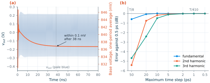
The time step. tran tstep tstop tstart tmax takes steps no longer than tmax, or than tstep and (tstop − tstart)/50 when tmax is left out. ngspice’s step control bounds the local truncation error of each step, but that tolerance is set for waveforms, not for harmonics 30 or 60 dB below the fundamental. Figure 2.3b shows the harmonics at −20 dBm against the largest step allowed. With 50 ps steps (eight points per period, what tran 50p 80n gives) the fundamental is 0.59 dB low and the second and third harmonics 5.41 and 4.67 dB low. At 10 ps the errors are 0.02, 0.18 and 0.48 dB; at 1 ps they are below 0.003 dB. A rule that held here: 30 to 40 steps per period of the highest harmonic you want to read to 0.1 dB.
The steady state. The bias of a nonlinear circuit moves when the signal is applied. The base–emitter junction rectifies: at −20 dBm the average collector current rises from 2.00 to 4.11 mA, and the base voltage, fed through \(R_B\), falls from 842.2 to 836.7 mV (Figure 2.3a). It settles to within 0.1 mV only after 38 ns, about 94 periods. A spectrum taken earlier mixes the start-up into the result.
The Fourier transform. A discrete Fourier transform of a record of length \(T_{rec}\) has bins \(\Delta f = 1/T_{rec}\) apart, and it treats the record as one period of a periodic signal. If the record holds an integer number \(M\) of periods of every tone,
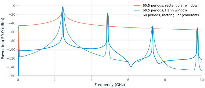
\[\Delta f = \frac{1}{T_{rec}}, \qquad T_{rec} = \frac{M}{f_0}, \tag{2.5}\]each tone falls exactly on a bin: coherent sampling. Otherwise the record’s ends do not meet, the tone’s energy leaks into every bin, and a tone between two bins reads low (Figure 2.4) [40]. Over 60.5 periods with a rectangular window, the fundamental reads −6.10 dBm instead of −2.17 dBm, and the leakage floor halfway to the second harmonic is at −41.3 dBm. A Hann window tapers the record’s ends: the floor falls to −101 dBm, but the fundamental still reads 1.4 dB low (−3.59 dBm). Sixty whole periods with no window give −2.17 dBm and a floor below −97 dBm; what remains there is the last of the start-up. ngspice offers both routes: fourier 2.44g v(out) fits the last period of the run (the tran deck above prints the harmonics and the THD), and linearize, set specwindow=hanning and fft v(out) give a windowed spectrum of the whole run. The figures of this chapter take the record into Python instead.
Common pitfall · Trusting the default time step
tran 50p 80nlooks harmless: 50 ps is a fine print step. But it is also the largest step ngspice will take, eight per period at 2.44 GHz, and the second harmonic comes out 5.4 dB too low with no warning. Always givetmax(the fourth argument) for RF transients, and check a harmonic by halving it.
2.5 Harmonic balance in Xyce
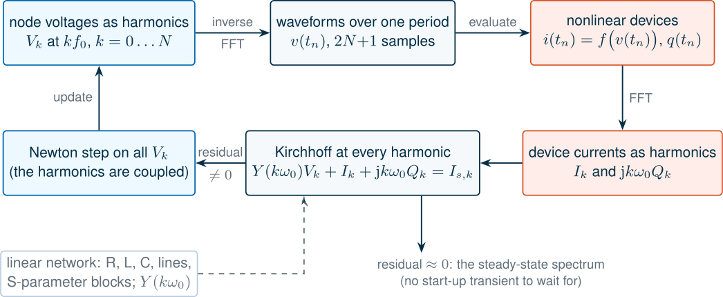
A transient finds the steady state by waiting for it. Harmonic balance (HB) looks for it directly [34, 33, 35]. If the circuit is driven at \(f_0\), every node voltage in the steady state is periodic and can be written as a sum of harmonics, truncated at the \(N\)-th:
\[v(t) = \sum_{k=-N}^{N} V_k\,e^{\,\mathrm{j}k\omega_0 t}, \qquad V_{-k} = V_k^*. \tag{2.6}\]The unknowns are the complex amplitudes \(V_k\). The linear part of the circuit (resistors, inductors, capacitors, lines, even measured S-parameter blocks) is described exactly at each harmonic by its admittance \(Y(k\omega_0)\). The nonlinear devices are evaluated in the time domain: an inverse FFT turns the \(V_k\) into waveforms at \(2N+1\) instants of one period, the device equations give the currents \(i(t)\) and charges \(q(t)\), and an FFT turns them back into harmonics \(I_k\) and \(Q_k\). Kirchhoff’s current law must then hold at every harmonic,
\[Y(k\omega_0)\,V_k + I_k + \mathrm{j}k\omega_0 Q_k - I_{s,k} = 0, \qquad k = 0 \dots N, \tag{2.7}\]where \(I_{s,k}\) are the sources. Newton’s method adjusts all the \(V_k\) together until the residual vanishes (Figure 2.5). The cost grows with the number of harmonics, not with the ratio of time scales; a linear circuit is solved in one step; and there is no start-up transient. For two tones \(f_1\) and \(f_2\), the frequencies are the mixing products \(m f_1 + n f_2\); Xyce keeps those with \(\vert m\vert\) and \(\vert n\vert\) up to the two values of numfreq and \(\vert m\vert + \vert n\vert \le\) intmodmax, 57 frequencies (including DC) for numfreq=7,7 intmodmax=7.
This is the complete Xyce deck for a single-tone power sweep, from −40 to 0 dBm in 1 dB steps:
* Chapter 2 running example in Xyce: single-tone harmonic balance, input power sweep
.lib /foss/pdks/ihp-sg13g2/libs.tech/xyce/models/cornerHBT.lib hbt_typ
.param pin=-40
.param va={sqrt(8*50*1e-3*pow(10, pin/10))}
VCC   vcc  0    1.2
VBB   bb   0    0.845
RB    bb   b    1k
XQ1   c    b    0 0 npn13G2 Nx=4
LC    vcc  c    100n
RC    vcc  c    150
CB1   in   m1   10p
L1    m1   b    14.5n
C1    b    0    235f
C2    c    0    489f
L2    c    m2   5.22n
CB2   m2   out  10p
VS    src  0    SIN(0 {va} 2.44e9)
RS    src  in   50
RLOAD out  0    50
.hb 2.44e9
.options hbint numfreq=8 startupperiods=4
.step pin -40 0 1
.print hb_fd v(out)
.end
numfreq=8 keeps eight harmonics; startupperiods=4 runs four periods of transient to make the initial guess. .print hb_fd writes the complex amplitude of v(out) at every frequency, from −8\(f_0\) to +8\(f_0\) (Xyce prints the two-sided spectrum, so a one-sided peak amplitude is twice the printed value), one block per step. The two-tone deck, ch02_amp_hb2.cir, adds a second source at 2.442 GHz in series, lists both frequencies on the .hb line and sets numfreq=7,7 intmodmax=7.
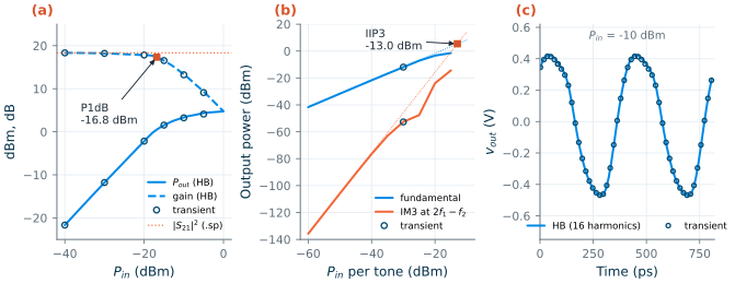
.sp. (b) Two-tone test at 2.440 and 2.442 GHz: fundamental and IM3 at 2f1 − f2, with the slope-1 and slope-3 extrapolations from −60 dBm and a 560 ns transient at −30 dBm (circles). (c) Output waveform at Pin = −10 dBm, 3 dB into compression.Figure 2.6a shows the single-tone sweep. At −40 dBm HB gives a gain of 18.33 dB, within 0.03 dB of .sp. The gain compresses by 1 dB at an input power of P1dB = −16.8 dBm (+0.5 dBm at the output), and the output saturates near +4.8 dBm. On the way, the average supply current rises from 2.03 to 10.24 mA: the voltage-biased junction pulls more DC current the harder it is driven, the effect seen in the transient of Section 2.4.
For the two-tone test, Figure 2.6b, the tones are two Bluetooth channels, 2.440 and 2.442 GHz. The third-order products at \(2f_1 - f_2\) = 2.438 GHz and \(2f_2 - f_1\) = 2.444 GHz fall inside the band, where no filter can remove them (Chapter 4). At low power the IM3 power rises with a slope of 3.00 dB/dB, and the intercept follows from one point,
\[\mathrm{IIP3} = P_{in} + \tfrac{1}{2}\left(P_{fund} - P_{IM3}\right), \tag{2.8}\]IIP3 = −13.0 dBm (OIP3 = +5.4 dBm) from the −60 dBm point. The same formula applied at −30 dBm gives −9.7 dBm: there the IM3 curve has left its slope of 3, and the extrapolation is no longer an intercept. At −10 dBm per tone, 3 dB beyond P1dB, the two-tone HB did not converge with these options; the single-tone sweep converged to 0 dBm.
Table 2.2. The same amplifier by every analysis (ngspice and Xyce in IIC-OSIC-TOOLS 2026.10, 27 °C).
| Quantity | Analysis | Result |
|---|---|---|
| \(\vert S_{21}\vert\) at 2.44 GHz | ngspice .sp / .ac with Eq. (2.1) |
18.355 / 18.355 dB |
Xyce .LIN |
18.34 dB | |
| Gain at Pin = −40 dBm | Xyce HB / ngspice transient | 18.33 / 18.33 dB |
| Gain at Pin = −10 dBm | Xyce HB / ngspice transient | 13.34 / 13.24 dB |
| Harmonics at −20 dBm (H1, H2, H3) | Xyce HB | −2.18, −17.67, −46.21 dBm |
| ngspice transient (1 ps) | −2.17, −17.66, −46.26 dBm | |
| Fundamental, IM3 at −30 dBm per tone | Xyce HB | −11.96, −52.60 dBm |
| ngspice transient (560 ns) | −11.95, −52.67 dBm | |
| Noise figure at 2.44 GHz | ngspice .sp / .noise |
3.569 / 3.569 dB |
Xyce .NOISE |
3.45 dB |
Table 2.2 collects the overlaps. Wherever two analyses can answer the same question, they agree to a few hundredths of a decibel at low drive and to about 0.1 dB in compression; the waveforms at −10 dBm differ by 6.2 mV rms on a 0.89 V peak-to-peak swing (Figure 2.6c). The difference is in the cost. The two-tone transient had to run 560 ns at 1 ps steps (560 000 points) to reach a steady state and hold one full 500 ns beat period for a coherent FFT; it took 15 s, against 2.6 s for one two-tone HB point (Table 2.4).
2.6 Periodic steady state and transient noise
Harmonic balance is one way to find a periodic steady state (PSS). The other is the shooting method [36]: guess the state of the circuit at the start of a period, simulate one period of transient, and use Newton’s method on the difference between the final and the initial state until the period closes on itself. ngspice-47 has a .pss analysis of this kind, written for autonomous circuits, oscillators, whose frequency is itself an unknown:
* van der Pol LC oscillator
L1 t 0 1n
C1 t 0 4.3p IC=0.1
R1 t 0 500
B1 t 0 I = -4m*v(t) + 4m*v(t)*v(t)*v(t)
.control
pss 2.4e9 30e-9 t 128 7 50 1e-3 uic
.endc
The arguments are the guessed frequency, a stabilization time of plain transient before the shooting starts, the node that sets the period, the number of points per period, the number of harmonics, the iteration limit and the steady-state tolerance. With a 30 ns stabilization time, .pss finds 2.4269 GHz and an amplitude of 0.817 V, matching the tank’s resonance (2.4271 GHz), a 200 ns transient (0.817 V) and the describing-function estimate of the amplitude (0.816 V). With 10 ns it reports convergence at 2.4282 GHz and 0.652 V, a wrong answer that looks like a right one: the shooting only polishes a state that the transient has nearly reached. On the driven amplifier, .pss changes its frequency guess to 4.19 GHz and aborts (“Cannot find a minimum for error vector in estimated period. Try to adjust tstab!”). For driven circuits, use HB in Xyce; for oscillators, check .pss against a long transient. Chapter 11 returns to oscillators.
Xyce adds the multi-time PDE (MPDE) method [37, 38], which gives a slow and a fast time variable to circuits with two widely separated time scales, such as a carrier and its modulation. Driven by one tone at −36 dBm, the amplifier’s output amplitude from .mpde 100p 20n with .options mpdeint n2=32 oscsrc=VS diff=1 is 41.1 mV, against 41.2 mV from HB. With the default fast-time differences (no diff=1) it is 25.0 mV, and 31.5 mV with 64 points: the default backward differences damp the resonant matching networks numerically.
What neither simulator offers is noise in a large-signal steady state: the periodic noise analyses that give the noise figure of a mixer or the phase noise of an oscillator. Xyce rejects .NOISE together with .HB (“Analysis type HB and print type NOISE are inconsistent”), and ngspice has no periodic noise analysis. For mixers and oscillators that leaves transient noise, below, and hand analysis.
Transient noise
ngspice can add noise to a transient through independent sources: trnoise(NA NT NALPHA NAMP) draws a Gaussian sample of rms value NA every NT seconds (the last two parameters add an optional 1/f part) and interpolates linearly between samples. Its one-sided density is flat, \(2\,\mathrm{NA}^2\,\mathrm{NT}\), well below \(1/\mathrm{NT}\), so a white density \(S\) needs
The linear interpolation also lowers the rms value measured on the waveform: trnoise(20u 10p 0 0) gives 16.51 µV, 0.825 of NA. Nothing else is noisy in a transient: a 1 kΩ resistor alone gives exactly 0 V rms, and so do the transistor models. The set enable_noisy_r line in the IIC-OSIC-TOOLS .spiceinit concerns .noise, not .tran: it makes behavioural resistors (r='expression') noisy, 4.071 nV/√Hz for 1 kΩ with it and 4.07 pV/√Hz (only the 1 GΩ feed) without it.
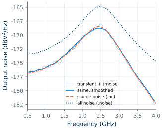
Figure 2.7 puts a trnoise source in series with the amplifier’s 50 Ω source, NA = 287.9 µV and NT = 5 ps for \(4kTR_S\), and runs a 2 µs transient. The output spectrum, estimated by averaging over many 20 ns segments (Welch’s method), follows the source noise predicted from the .ac gain within 0.1 dB in the band. The total output noise from .noise is 3.57 dB higher, the noise figure: the transient sees only the noise we put in.
.ac, and the total noise from .noise.Table 2.3. What the simulators in IIC-OSIC-TOOLS 2026.10 do with RF circuits, as tested for this chapter.
| Capability | ngspice-47 | Xyce 7.10 |
|---|---|---|
| DC, AC, noise | yes; port resistance noiseless in .noise |
yes; .NOISE lists every source |
| S-parameters | .sp, with noise figure and noise parameters |
.LIN, S-parameters only; Touchstone 2.0 (data order 12_21) or 1.0 output |
| Harmonic balance | no | .HB, one and several tones; two tones failed 3 dB past P1dB |
| Periodic steady state | .pss, oscillators only; result depends on the stabilization time |
through .HB (driven circuits) |
| Multi-time (MPDE) | no | .MPDE; correct only with diff=1 |
| Noise in a large-signal steady state | no | no (.HB with .NOISE rejected) |
| Transient noise | trnoise/trrandom sources only; resistors and devices noiseless |
TRNOISE accepted but gives no noise |
| Spectra | fourier, fft with specwindow |
.FFT |
2.7 Electromagnetic simulation with openEMS and Palace
Circuit simulators take the passives as given. An EM solver computes them from the layout and the metal stack, solving Maxwell’s equations, and returns S-parameters to put back into the circuit. Two methods dominate the open-source tools.
The finite-difference time-domain (FDTD) method [42] of openEMS divides space into a rectilinear grid of cells, places the electric and magnetic field components on staggered (Yee) positions, and steps them forward in time. One run with a broadband Gaussian pulse gives the response at all frequencies, through a Fourier transform of the port voltages and currents; microstrip dispersion was among its first applications [43]. The explicit time step is limited by the smallest cell (the Courant condition),
\[\Delta t \le \frac{1}{c\sqrt{\Delta x^{-2} + \Delta y^{-2} + \Delta z^{-2}}}, \tag{2.10}\]so the thin layers of an IC metal stack (cells of 0.4 µm) force femtosecond steps, 1.16 fs here, and long runs for high-Q structures whose energy decays slowly.
The finite-element method (FEM) [15] of Palace divides the structure into tetrahedra that follow its shape, from thin metal sheets to curved spirals, and solves the frequency-domain equations at each frequency as a large sparse linear system, distributed over many processors with MPI. It handles fine features and resonant structures well, but each frequency point is a solve (Palace can also sweep adaptively). IHP’s flows [198] read a GDS layout and an XML description of the SG13G2 stack for both solvers: gds2openEMS-style Python scripts for openEMS, and gds2palace, which meshes with gmsh and writes Palace’s JSON configuration.
We ran IHP’s run_line_viaport example in openEMS, which the workflow’s user guide walks through along with the meshing and port choices behind it [204]: an 880 µm long, 15 µm wide TopMetal2 line over a Metal1 ground plane (a microstrip), with via ports from Metal1 to TopMetal2 at both ends and the stack without the substrate, which the ground plane shields. The script tools/em/ch02_line.py keeps IHP’s settings (1 µm cells on the conductors, 0–110 GHz, end at −40 dB of energy), writes the results into the repository, and skips the 3D viewer. The mesh has 303 264 cells, and the run took 252 s on four threads.
The same layout went through IHP’s Palace flow, palace_line_viaport (tools/em/ch02_line_palace.py): gmsh meshed it into 97 835 tetrahedra in 17 s. With IHP’s settings, second-order elements (674 724 unknowns) and an adaptive sweep, the solve had not finished after 47 minutes on four processes of a laptop shared with other jobs, so we switched to first-order elements (130 639 unknowns) at six frequencies, which took 637 s on two processes.
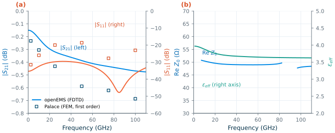
Figure 2.8 shows the result. The line is matched to 50 Ω (\(\vert S_{11}\vert\) ≤ −29.5 dB up to 110 GHz; Re \(Z_0\) = 50.4 Ω at 10 GHz and 49.0 Ω at 50 GHz). It loses 0.155 dB at 2.44 GHz and 0.388 dB at 50 GHz, 0.176 and 0.441 dB/mm: the series resistance, 1.74 Ω at DC, grows with the skin effect. The effective permittivity, from the phase of \(S_{21}\), falls from 3.97 at 2.44 GHz to 3.66 at 50 GHz, below the oxide’s because part of the field is in the air above the line. The via ports add a small inductance that IHP’s flow does not de-embed, and it is included in these numbers. Palace agrees on the character of the line but not on the details: it gives 0.234 dB of loss at 2.44 GHz and 0.589 dB at 50 GHz, and \(\vert S_{11}\vert\) = −18.6 dB at 50 GHz where openEMS gives −30.6 dB. The two runs differ in their discretization, 1 µm cells against first-order elements on IHP’s coarser mesh, and in their port models; only a refinement study of each, the subject of Chapter 7, would say which is closer. Chapter 18 later made that check for Palace on a TopMetal2 line: at 50 GHz first-order elements gave a characteristic impedance 14 % low and 17 % more loss than second-order elements, which agree with a finer reference within 2 %. The first-order Palace points here are therefore the less trustworthy of the two, and their extra loss is the error that check predicts. An EM result without a mesh-convergence check is a number, not an answer. Chapter 7 simulates inductors and transformers in depth, and Chapter 18 puts EM results back into a circuit.
2.8 Post-processing in Python
Every analysis above ends in numbers that need maths: Eq. (2.1) for S21, Eq. (2.2) for the noise figure, an FFT for the spectra, the stability factors and gains of Chapter 3. The course’s helpers in tools/rfic do this for every chapter. A short session:
import sys; sys.path.insert(0, "tools")
from rfic.spice import run, xyce
from rfic.rf import sp_matrix, freq, db, stability, hb_tone, vpk2dbm, read_snp

res = run(netlist_lines, "sg13g2", ["op", "sp lin 351 0.5e9 4e9 1"], libs=("hbt",))
S = sp_matrix(res["sp1"])                  # S[f, 2, 2] from s_1_1 ... s_2_2
f = freq(res["sp1"])
K, mu = stability(S)                       # Rollett K and the mu factor
nf = res["sp1"]["nf"].real                 # dB

hb = xyce(xyce_lines, libs=("hbt",))       # .hb / .print hb_fd lines inside xyce_lines
p_out = vpk2dbm(hb_tone(hb["hb_fd"], "v(out)", 2.44e9))   # dBm into 50 ohm
f_em, S_em, z0 = read_snp("tools/em/ch02_line.s2p")
run() writes the netlist with the PDK’s model libraries, runs ngspice (in the IIC-OSIC-TOOLS container when the PDK is not installed locally) and returns one dictionary per analysis; xyce() does the same for Xyce and parses its .prn files; tone_powers() takes the harmonics from the end of a transient by resampling an integer number of periods, the coherent sampling of Section 2.4.
A Touchstone file stores S-parameters against frequency as text [188]. Its option line # Hz S RI R 50 gives the frequency unit, the parameter type, the number format (RI real–imaginary, MA magnitude–angle in degrees, DB dB–angle) and the reference impedance; each line then holds a frequency and the parameters, in the order S11, S21, S12, S22 for a version 1.0 two-port. The file extension gives the number of ports: .s1p, .s2p, .s4p. read_snp() reads version 1.0 files; the chapter’s script has a small reader that honours the version 2.0 keywords Xyce writes. Appendix B (RF simulation cheat sheet) lists the syntax of every analysis used here.
2.9 Choosing the right analysis
Table 2.4 gives the cost of each analysis of the running example, as reported by the simulators themselves (the start of the Docker container is not included). Other jobs on the same machine moved the times by up to a factor of three: the one-tone transient took between 1.5 and 4.7 s in different runs.
Table 2.4. Run time of each analysis of the running example (simulator-reported; the shortest of three runs, single runs for the sweeps, the transient noise and the EM solvers; IIC-OSIC-TOOLS 2026.10 under Docker on an Apple M2 laptop).
| Analysis | Tool | Size | Time |
|---|---|---|---|
| Operating point | ngspice .op |
1 point | 7 ms |
| AC | ngspice .ac |
351 frequencies | 2 ms |
| Noise | ngspice .noise |
351 frequencies | 6 ms |
| S-parameters with noise | ngspice .sp |
351 frequencies | 18 ms |
| S-parameters | Xyce .LIN |
351 frequencies | 0.17 s |
| Transient, one tone | ngspice .tran |
80 ns, 1 ps steps | 3 s |
| Transient, two tones | ngspice .tran |
560 ns, 1 ps steps | 15 s |
| Harmonic balance, one tone | Xyce .HB |
8 harmonics, one power | 0.25 s |
| — power sweep | Xyce .HB |
41 powers | 18 s |
| Harmonic balance, two tones | Xyce .HB |
57 frequencies, one power | 2.6 s |
| — power sweep | Xyce .HB |
10 powers | 47 s |
| Multi-time | Xyce .MPDE |
32 fast points, 20 ns slow | 0.85 s |
| Periodic steady state (oscillator) | ngspice .pss |
30 ns + shooting | 2.3 s |
| Transient noise | ngspice .tran |
2 µs, 5 ps steps | 51 s |
| EM, FDTD | openEMS | 303 k cells, 4 threads | 252 s |
| EM, FEM | Palace | 131 k unknowns, 6 frequencies, 2 processes | 637 s |
Table 2.5 turns the chapter into a guide. The small-signal analyses cost milliseconds and answer most questions about gain, match, stability and noise; harmonic balance answers the large-signal questions about a driven circuit at a fraction of a transient’s cost, the more so the closer its tones; the transient remains the analysis of last resort and of first check, and the only one for start-up, switching and signals that are not periodic.
Table 2.5. Which analysis answers which question.
| Question | Analysis | Tool | Watch out for |
|---|---|---|---|
| Is the bias right? | .op |
ngspice | every small-signal result depends on it |
| Gain, match, isolation, stability | .sp (.ac with Eq. 2.1) |
ngspice; Xyce .LIN |
ports must be at the reference planes you care about |
| Noise figure and noise parameters | .sp with noise; .noise with a summary |
ngspice | NF referred to the simulation temperature; port resistance noiseless |
| Which element adds the noise | .noise with points per summary |
ngspice, Xyce | — |
| Compression, harmonics, output power, efficiency | .HB, single tone, power sweep |
Xyce | enough harmonics; convergence in deep compression |
| Intermodulation, IIP3 | .HB, two tones |
Xyce | extract IIP3 where the slopes are 1 and 3 |
| Start-up, settling, switching, non-periodic signals | .tran |
ngspice | tmax; wait for the steady state; coherent FFT |
| Oscillator frequency and amplitude | .tran; .pss |
ngspice | .pss needs a long enough stabilization time |
| Noise with large signals (mixer NF, phase noise) | .tran with trnoise sources |
ngspice | only the sources you add are noisy; no periodic noise analysis |
| Passives, lines, interconnect | FDTD; FEM | openEMS; Palace | mesh size and run time; de-embed the ports |
Try it · The chapter script
Every number in this chapter comes from
tools/figs/ch02_rfsim.py(python3 tools/figs/ch02_rfsim.py small tran hb), and the four decksch02_amp*.cirrun as listed in IIC-OSIC-TOOLS. Three experiments: (1) raiseRBto 2 kΩ at the top of the script (thedesignpart finds the new \(V_{BB}\) for 2 mA and redesigns the L-sections) and rerundesign small --resim: how much of Table 2.1 moves, and what happens to the noise figure? Then try 5 kΩ: why does thedesignpart stop? (2) Inch02_amp_tran.cir, changetran 1p 80n 0 1ptotran 50p 80nand compare thefourieroutput with Table 2.2. (3) Inch02_amp_hb.cir, setnumfreq=3: at which input power does the output differ from the 8-harmonic result by 0.1 dB?
- One netlist with ngspice ports serves
.op,.ac,.noiseand.sp; they agree to the third decimal (18.355 dB, 3.569 dB) once the noiseless port resistance and Eq. (2.1) are accounted for. ngspice refers the noise figure to the simulation temperature, not to 290 K.- A noise analysis with a summary names the noisy element: here the 1 kΩ bias resistor adds 43 % of the output noise.
- A transient spectrum needs a small
tmax(50 ps steps lost 5.4 dB on the second harmonic), a settled steady state (38 ns here) and a coherent record or a window.- Harmonic balance in Xyce gives P1dB (−16.8 dBm) and IIP3 (−13.0 dBm) directly, agrees with the transient to about 0.1 dB, and costs a fraction of it for closely spaced tones.
- ngspice’s
.pssis for oscillators and needs checking; neither simulator has periodic noise; transient noise contains only trnoise sources.- FDTD (openEMS) and FEM (Palace) turn layouts into S-parameters; IHP’s TopMetal2 line is a 50 Ω microstrip losing 0.18 dB/mm at 2.44 GHz in openEMS, and the two solvers’ disagreement of up to 0.2 dB shows why every EM result needs a mesh-convergence check.
Further reading
- K. S. Kundert, “Introduction to RF simulation and its application” [32]: the classic tutorial on harmonic balance, shooting and periodic small-signal and noise analyses, the ones the commercial simulators have and the open-source ones mostly lack.
- K. S. Kundert and A. Sangiovanni-Vincentelli [33] and V. Rizzoli and A. Neri [35]: how harmonic balance works inside, and how microwave engineers used it.
- J. Roychowdhury [38]: the multi-time formulation behind Xyce’s MPDE.
- F. J. Harris [40]: everything about windows and leakage.
- The ngspice manual [194] (chapters on
.sp,.pssand transient noise), the Xyce Users’ and Reference Guides [195] (.HB,.LIN,.MPDE), and IHP’s openEMS and Palace workflows [198] with their documentation; for openEMS, V. Mühlhaus’s user guide [204] explains FDTD time steps, simulation boundaries, meshing and ports for the SG13G2 stack, step by step.