Chapter 15
Digital PLLs and Clock Recovery
A digital PLL replaces the charge pump and its large loop-filter capacitor by a time-to-digital converter, a few adders and a digitally controlled oscillator. This chapter builds the pieces for the course radio: an inverter-chain TDC whose resolution we simulate in SG13G2, a DCO made from the Chapter 11 tank with switched capacitor banks, and the z-domain loop that joins them. It then turns to the loops that use a single bit of phase information, bang-bang PLLs and clock and data recovery, and to the delay-locked loop. The result is an illustrative all-digital PLL that meets the course's phase-noise specification at 1 MHz with 8.9 dB to spare, and whose in-band noise is set, almost exactly at the budget, by one inverter delay.
- Explain what an all-digital PLL replaces in a charge-pump PLL, and describe it in the phase domain with a frequency control word.
- Derive the in-band phase-noise floor of a TDC from its resolution, and simulate the resolution of an inverter-chain TDC and its supply and temperature sensitivity.
- Calculate the frequency step of a capacitor-bank DCO and the phase noise of its quantization, with and without delta-sigma dithering.
- Model a type-II digital loop in the z-domain, choose its proportional and integral gains, and check the model with a time-domain simulation.
- Explain how bang-bang phase detectors, delay-locked loops and clock-and-data-recovery loops work, and estimate the effective gain of a bang-bang detector and the jitter tolerance of a bang-bang CDR.
Contents
15.1 Why digital PLLs
The PLL chapter of The Art of Analog IC Design and Chapter 12 of this course build the classic charge-pump PLL: a phase-frequency detector turns the phase error into current pulses, a passive loop filter integrates them on a capacitor, and the capacitor’s voltage tunes the VCO. The loop filter is the awkward part. For a charge-pump loop around the course VCO with a 200 kHz bandwidth, a 100 µA charge pump, the Chapter 11 tuning gain of 108 MHz/V, a division ratio of 122.1 and the stabilizing zero at a quarter of the crossover frequency, the filter needs R = 14.2 kΩ and C1 = 224 pF: 0.149 mm² of MIM capacitor at 1.5 fF/µm² (Chapter 7), and the capacitance grows as the square of the inverse bandwidth. The capacitor’s leakage, the charge pump’s current mismatch and the varactor’s dependence on the tuning voltage all add their own errors.
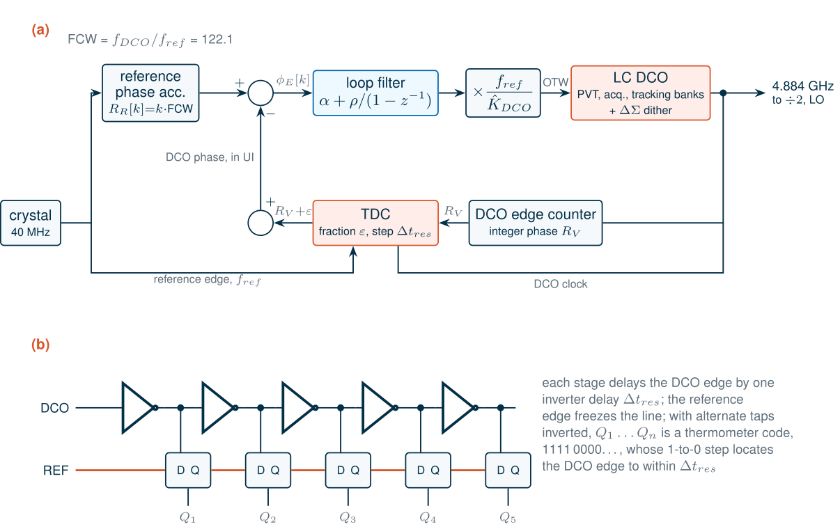
An all-digital PLL (ADPLL) keeps the loop and changes every block on it (Figure 15.1a) [153, 154]. Phase is counted in units of the oscillator period, the unit interval (UI). A reference phase accumulator adds the frequency control word FCW = fDCO/fref once per reference cycle; a counter of the oscillator’s edges gives its integer phase \(R_V\) and a time-to-digital converter (TDC) measures the fraction \(\varepsilon\) at each reference edge. Their difference is the phase error,
\[\text{FCW} = \frac{f_{DCO}}{f_{ref}}, \qquad \phi_E[k] = k\cdot\text{FCW} - \big(R_V[k] + \varepsilon[k]\big), \tag{15.1}\]a number. A digital filter turns it into an oscillator tuning word (OTW) for a digitally controlled oscillator (DCO), an LC oscillator tuned by switched capacitors instead of a varactor. The filter is a few adders and registers, so its bandwidth is set by programmable coefficients, it costs no area, it does not leak, and it can change its own bandwidth during acquisition. Fractional-N operation needs no divider or delta-sigma modulator in the loop: FCW is simply a fractional number. For the course channel at 2442 MHz the DCO runs at 4.884 GHz and FCW = 122.1. The price is quantization: the TDC measures time in steps of \(\Delta t_{res}\) and the DCO changes frequency in steps of \(\Delta f_{res}\), and both steps become noise.
15.2 Time-to-digital converters
The inverter-chain TDC
The simplest TDC is a delay line sampled by flip-flops (Figure 15.1b). The DCO edge runs down a chain of inverters; the reference edge clocks a flip-flop at every tap at once, freezing the line. With every other tap inverted, the flip-flops hold a thermometer code whose step marks how far the DCO edge has travelled: the time from the DCO edge to the reference edge, to within one inverter delay \(\Delta t_{res}\) [155]. Two such measurements, on a rising and a falling DCO edge, give the period \(T_V\) in units of \(\Delta t_{res}\) as well, and the fraction \(\varepsilon\) is the measured delay divided by that period. To cover a whole period the line needs
\[N_{stages} \ge \frac{T_V}{\Delta t_{res}} = \frac{1}{f_{DCO}\,\Delta t_{res}} \tag{15.2}\]stages in the fastest corner.
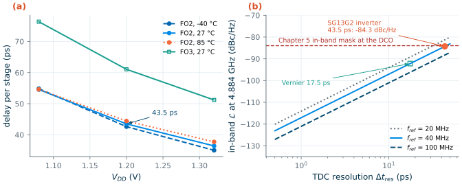
We simulated the delay line in ngspice: twelve SG13G2 inverters (lv MOS, Wn/Wp = 1/2 µm, L = 0.13 µm), each driving the next stage and one sampler input (fan-out of two, FO2), at three supplies and three temperatures (Figure 15.2a). At 1.2 V and 27 °C one stage takes 43.5 ps (45.1 ps falling, 41.9 ps rising). The supply dominates the spread: from 1.08 to 1.32 V the delay falls from 54.5 to 36.4 ps, 1.74 % per 10 mV. Temperature hardly matters at this supply (0.0146 ps/°C), because the falling threshold voltage and the falling mobility nearly cancel. Over all nine corners the delay spans 35.0–54.8 ps, a ratio of 1.57. The DCO period at 4.884 GHz is 205 ps, so a nominal line spans one period in 4.71 stages and the fastest corner needs 5.85: an eight-stage line is enough, and the TDC resolves only about five levels per DCO cycle.
The spread is why an ADPLL measures its TDC’s gain continuously, by averaging the measured period, and normalizes \(\varepsilon\) with it [154]; Section 15.6 shows the alternative of locking the delay line with a DLL. A finer resolution than one gate delay needs a Vernier TDC: two delay lines with stage delays \(\tau_1 > \tau_2\), the start edge in the slow line and the stop edge in the fast one, whose difference \(\tau_1 - \tau_2\) is the resolution [156]. Loading the same inverters with two samplers instead of one (FO3) gives 61.0 ps per stage, so a Vernier pair of FO3 and FO2 lines resolves 17.5 ps, at the price of more stages, a longer conversion and a resolution that is now a small difference of two large, mismatched delays.
Quantization noise and the in-band floor
The TDC rounds the time error to a multiple of \(\Delta t_{res}\). If the error is “busy”, varying by many steps from one reference edge to the next, the rounding error is uniform over one step, white, and uncorrelated with the signal. Converted to phase of the DCO and spread over the band sampled at \(f_{ref}\), it gives
Key equation · In-band phase-noise floor of a TDC
\[\mathcal{L}_{TDC} = \frac{(2\pi)^2}{12}\left(\frac{\Delta t_{res}}{T_V}\right)^2\frac{1}{f_{ref}} = \frac{(2\pi\,\Delta t_{res}\,f_{DCO})^2}{12\,f_{ref}}, \tag{15.3}\]
referred to the DCO frequency [155]. Inside the loop bandwidth the loop copies the measured phase, noise included, to the output, so Eq. (15.3) is the ADPLL’s in-band floor.
Derivation · The TDC floor
The rounding error of the time measurement is uniform over \(\Delta t_{res}\), with variance \(\Delta t_{res}^2/12\). As a phase of the DCO it is \(2\pi\,\Delta t/T_V\), so its variance is \(\sigma_\phi^2 = (2\pi\Delta t_{res}/T_V)^2/12\) rad². One sample is taken per reference cycle, and a white sequence of variance \(\sigma_\phi^2\) sampled at \(f_{ref}\) has a two-sided spectral density \(\sigma_\phi^2/f_{ref}\) between \(-f_{ref}/2\) and \(f_{ref}/2\). The single-sideband phase noise is the two-sided density of the phase, \(\mathcal{L} = S_\phi^{(2)} = \sigma_\phi^2/f_{ref}\), which is Eq. (15.3). The floor falls by 3 dB per doubling of \(f_{ref}\) and rises by 6 dB per doubling of \(\Delta t_{res}\) or of \(f_{DCO}\).
For the simulated 43.5 ps at 40 MHz, Eq. (15.3) gives −84.3 dBc/Hz at 4.884 GHz, −90.3 dBc/Hz at the LO (Figure 15.2b). The course budget of Chapter 5 allows −90 dBc/Hz at the LO inside the loop bandwidth, −84.0 dBc/Hz at the DCO: the inverter TDC sits only 0.3 dB below it, and in the slowest corner (54.8 ps, −82.3 dBc/Hz) above it. The Vernier’s 17.5 ps gives −92.2 dBc/Hz. To stay 10 dB below the budget at 40 MHz the TDC would need 14.3 ps.
Common pitfall · Treating TDC quantization as white noise
Eq. (15.3) assumes the rounding error is random. In a quiet loop it is not: the DCO phase hardly moves between reference edges, and with FCW = 122.1 the fractional phase returns to the same ten values every ten cycles. The error then repeats, and its power appears as spurs at multiples of 4 MHz (Section 15.4), not as a floor. In an integer channel it is constant, and the TDC behaves like a one-bit detector (Section 15.5).
15.3 Digitally controlled oscillators
A DCO is an LC oscillator whose tank capacitance is a sum of switched units. A step \(\Delta C\) in a tank of capacitance \(C\) moves the frequency by
\[\Delta f = \frac{f}{2}\,\frac{\Delta C}{C}. \tag{15.4}\]The Chapter 11 tank (537 fF at 4.868 GHz) gives 4.53 kHz per attofarad. Its 4-bit bank, with an LSB of 32.6 MHz (7.19 fF), already covers process, voltage and temperature. An ADPLL adds finer banks below it [152]: an acquisition bank of 2 MHz steps (441 aF), used while the loop pulls in, and a tracking bank whose 250 kHz steps (55.2 aF) are thermometer-coded so that every code change is one small, glitch-free step. Steps of tens of attofarads are far below a MIM capacitor’s minimum; they are made from the difference between the two states of a small MOS varactor, or by placing a unit capacitor in series with a larger one. We do not design those cells here. Without an analog tuning node, the DCO also loses the varactor’s conversion of tuning-line noise into frequency noise; its supply sensitivity remains.
Quantization noise and dithering
The tracking word changes once per reference cycle, so the DCO frequency is the wanted frequency plus a rounding error uniform over \(\Delta f_{res}\), held for one period. Phase is the integral of frequency, which turns the white frequency error into phase noise falling at 20 dB per decade [152]:
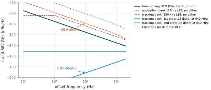
\[\mathcal{L}_{DCO,q}(\Delta f) = \frac{1}{12}\left(\frac{\Delta f_{res}}{\Delta f}\right)^2\frac{1}{f_{ref}}\,\mathrm{sinc}^2\!\left(\frac{\Delta f}{f_{ref}}\right). \tag{15.5}\]The 250 kHz tracking step gives −98.9 dBc/Hz at 1 MHz (Figure 15.3), 16.5 dB above the DCO’s own −115.4 dBc/Hz (the pessimistic end of the Chapter 11 estimate). Without help the step would have to shrink to 11.8 kHz, 2.6 aF. The help is dithering: a delta-sigma modulator clocked at \(f_d \gg f_{ref}\) toggles the tracking bank’s least significant unit so that its average carries the fractional part of the word, and shapes the rounding error to high frequencies (Chapter 14 treats the modulators). With an \(n\)-th-order modulator,
\[\mathcal{L}_{DCO,q}(\Delta f) = \frac{1}{12}\left(\frac{\Delta f_{res}}{\Delta f}\right)^2\frac{1}{f_d}\left[2\sin\frac{\pi\Delta f}{f_d}\right]^{2n}\mathrm{sinc}^2\!\left(\frac{\Delta f}{f_d}\right). \tag{15.6}\]At \(f_d\) = 640 MHz (16 fref, about fDCO/7.63), a first-order modulator flattens the noise to −151.1 dBc/Hz; a second-order one pushes it to −191.2 dBc/Hz at 1 MHz and −171.2 dBc/Hz at 10 MHz, negligible next to the oscillator.
15.4 The digital loop filter and the z-domain model
A type-II loop in the z-domain
The loop filter of Figure 15.1a is a proportional–integral filter: a gain \(\alpha\) in parallel with an accumulator of gain \(\rho\). The normalization block multiplies by \(f_{ref}/\hat K_{DCO}\), the inverse of the DCO’s measured gain, so a filter output of 1 changes the DCO frequency by exactly \(f_{ref}\), one UI per reference period. With one cycle of latency between the phase measurement and the DCO update, the open-loop gain in UI per UI is [154]
\[L(z) = \left(\alpha + \frac{\rho}{1-z^{-1}}\right)\frac{z^{-1}}{1-z^{-1}}. \tag{15.7}\]The second factor is the DCO, an integrator of frequency into phase. Two integrators make a type-II loop: like the charge-pump PLL with its capacitor, it tracks a frequency offset with zero phase error. Far below \(f_{ref}\), \(z^{-1}/(1-z^{-1}) \approx f_{ref}/s\), and the loop becomes the familiar continuous one (Chapter 12):
\[L(s) \approx \frac{\alpha f_{ref}}{s} + \frac{\rho f_{ref}^2}{s^2}, \qquad \omega_n = f_{ref}\sqrt{\rho}, \quad \zeta = \frac{\alpha}{2\sqrt{\rho}}, \quad f_c \approx \frac{\alpha f_{ref}}{2\pi}. \tag{15.8}\]The gains are usually powers of two, so the multipliers are shifts; with \(\alpha = 2^{-k}\) and \(\rho = 2^{-(2k+1)}\) the damping is 0.707. Like the charge-pump loop, the loop low-pass filters the TDC’s noise and high-pass filters the DCO’s:
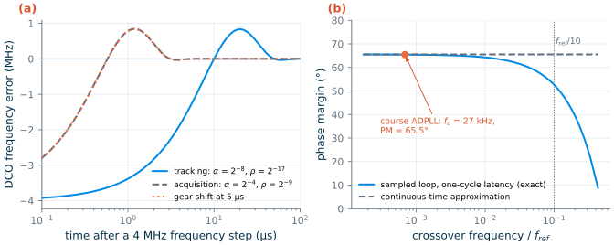
\[\mathcal{L}_{out} = \mathcal{L}_{TDC}\,\lvert H\rvert^2 + \left(\mathcal{L}_{DCO} + \mathcal{L}_{DCO,q}\right)\lvert 1-H\rvert^2, \qquad H = \frac{L}{1+L}. \tag{15.9}\]The loop is a sampled system, and the approximation fails as the bandwidth approaches \(f_{ref}\) (Figure 15.4b). The exact phase margin of Eq. (15.7) equals the continuous 65.5° for narrow loops but falls to 52.6° at a crossover of \(f_{ref}/10\), the usual limit for any sampled PLL [12].
An illustrative ADPLL for the course radio
Worked example 15.1 · Choosing the loop gains
With the simulated 43.5 ps TDC and the Chapter 11 DCO, Eq. (15.9) sets the bandwidth. A wide loop passes the TDC’s −84.3 dBc/Hz floor out to large offsets; a narrow one leaves the DCO’s 1/f² noise unsuppressed. Sweeping \(\alpha = 2^{-k}\) with \(\rho = \alpha^2/2\), the integrated phase error at the LO from 1 kHz to 8 MHz is smallest at \(\alpha = 2^{-8}\), \(\rho = 2^{-17}\): 0.807°, against 1.71° at \(\alpha = 2^{-5}\) (a 295 kHz loop) and 1.13° at \(\alpha = 2^{-10}\) (9.05 kHz). The chosen loop crosses over at 27.4 kHz, has a 3 dB bandwidth of 36.3 kHz, ζ = 0.707 and a 65.5° phase margin. The optimum lies near the offset where the TDC floor meets the free-running DCO noise, 27.9 kHz here. The 295 kHz loop would give −104.0 dBc/Hz at 1 MHz from the LO, 6 dB worse than the specification.
A 36 kHz loop is slow: it settles a 4 MHz channel step to 10 kHz in 78.3 µs (Figure 15.4a), half of the 150 µs that BLE leaves between packets [184]. Digital loops escape this trade by gear shifting: they start with wide gains (\(\alpha = 2^{-4}\), \(\rho = 2^{-9}\), a 442 kHz crossover), which settle the same step in 4.8 µs, and switch to the narrow gains once locked, here after 5 µs, keeping the accumulator’s state so that the switch disturbs nothing [153].
To check Eq. (15.9) we simulated the loop in the time domain at the reference rate: a TDC that rounds the DCO’s fractional phase to 43.5 ps, the PI filter, a tracking bank dithered by a second-order delta-sigma modulator at 640 MHz, and a DCO whose phase performs the random walk that gives −115.4 dBc/Hz at 1 MHz. This is a behavioural model, not a circuit: the TDC is ideal apart from its step, and the DCO’s gain is normalized exactly. Figure 15.5 shows the result for two cases. With a random offset added before the TDC and subtracted after it (a subtractive dither that makes the rounding error white, as Eq. (15.3) assumes), the simulated spectrum follows the linear model within 0.761 dB (median from 10 kHz to 10 MHz): −82.2 dBc/Hz in band against −80.8 dBc/Hz, and −112.8 dBc/Hz at 1 MHz in both. Without the dither, at FCW = 122.1, the pitfall of Section 15.2 appears: the in-band noise drops to −97.8 dBc/Hz, but spurs rise at multiples of 4 MHz, the largest −61.5 dBc at 4 MHz from the DCO, −67.5 dBc at 2 MHz from the LO, on top of the adjacent channel. These are the fractional spurs of Chapter 14 in a new form; real ADPLLs fight them with dither, finer TDCs, and digital cancellation of the predictable fractional phase.
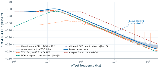
Table 15.1 collects the design. Reference noise is left out: a 40 MHz crystal is multiplied by FCW² in band, and Chapter 12 adds it to the budget.
Table 15.1. An illustrative ADPLL for the course radio at the 2442 MHz channel (DCO 4.884 GHz, FCW = 122.1), typical corner, 27 °C. Only the TDC delay is a transistor-level simulation; the rest is the behavioural and linear models of this chapter.
| Block or quantity | Choice | Result | Basis |
|---|---|---|---|
| TDC | flash, SG13G2 inverters 1/2 µm, FO2, ≥ 6 stages | Δtres = 43.5 ps (35.0–54.8 ps over ±10 % VDD, −40 to 85 °C) | ngspice |
| TDC in-band floor | Eq. (15.3) at 40 MHz | −84.3 dBc/Hz at the DCO (−90.3 at the LO); budget −84.0 | Eq. (15.3) |
| DCO | Chapter 11 tank; banks of 32.6 MHz, 2 MHz, 250 kHz | 4.53 kHz/aF; tracking LSB 55.2 aF | Eq. (15.4) |
| DCO dither | 2nd-order ΔΣ at 640 MHz | −191.2 dBc/Hz at 1 MHz (negligible) | Eq. (15.6) |
| Loop filter | α = 2−8, ρ = 2−17; acquisition α = 2−4, ρ = 2−9 | fc = 27.4 kHz, 65.5°; 4 MHz step settles in 4.8 µs with gear shift | z-domain model |
| Phase noise at 1 MHz | −112.8 dBc/Hz at the DCO (−118.9 at the LO); mask −104.0, margin 8.9 dB | model and time domain | |
| In-band (10 kHz) | −80.8 dBc/Hz at the DCO, 3.2 dB above the flat part of the mask | model | |
| Integrated phase error at the LO, 10 kHz–8 MHz | 0.753° (model), 0.664° (time domain); the mask itself gives 1.11° | model and time domain | |
| Fractional spur without TDC dither | FCW = 122.1 | −67.5 dBc at 2 MHz from the LO | time domain |
| Better TDC options | Vernier FO3/FO2; bang-bang PD (Section 15.5) | 17.5 ps: −92.2 dBc/Hz; BBPD: −123.2 dBc/Hz equivalent | ngspice; Eq. (15.11) |
What this means for your design
In SG13G2 at 40 MHz, one inverter delay is just good enough for the course radio: the loop meets −110 dBc/Hz at 1 MHz from the LO, and its integrated phase error is below what Chapter 5’s mask assumed, but the in-band noise has no margin and rises above the mask in the slow corner. Every improvement attacks Eq. (15.3): a finer TDC (Vernier, or interpolating between two lines), a faster reference (80 MHz buys 3 dB), or no multi-bit TDC at all, which is where the next section goes.
15.5 Bang-bang PLLs
A bang-bang phase detector (BBPD) is a single flip-flop: the reference edge samples the DCO clock, and the output says only whether the DCO is early or late. It is the extreme TDC, one bit with no dead zone, and it is fast, small and free of the delay line’s PVT spread. Its gain depends on the jitter. With no noise, a loop around it never settles: the DCO is always pushed one way or the other, and the phase error circulates in a limit cycle whose size is set by the proportional step and the loop latency [157]. With random jitter of rms value \(\sigma\) (in UI) at its input, the detector’s average output against a small phase error \(\phi\) is \(\mathrm{erf}\big(\phi/(\sqrt{2}\,\sigma)\big)\), a straight line near zero with the slope
\[K_{BB} = \sqrt{\frac{2}{\pi}}\,\frac{1}{\sigma} \tag{15.10}\]per UI. The rest of the detector’s output, the difference between its ±1 and that straight line, behaves as a white noise source referred to its input of variance \((\pi/2 - 1)\sigma^2\) [157], which gives a floor like Eq. (15.3):
\[\mathcal{L}_{BB} = (2\pi)^2\left(\frac{\pi}{2}-1\right)\frac{\sigma^2}{f_{ref}}. \tag{15.11}\]We simulated a bang-bang version of the course loop in the time domain: the same DCO noise, a proportional step of \(2^{-14}\) UI (12.5 fs of DCO phase per decision) and \(\rho = 2^{-20}\) (Figure 15.6). Without noise the phase error cycles with a period of 8.08 reference cycles and a peak-to-peak size of 50.4 fs. With the DCO’s random walk (55 fs per reference period) the jitter at the detector is σ = 190 fs, so Eq. (15.10) gives KBB = 861 per UI and the linearized loop a bandwidth of 443 kHz; the simulated jitter transfer has its 3 dB point at 472 kHz. With a DCO 12 dB noisier, σ grows to 3.14 ps, KBB falls to 52 and the bandwidth to 72.3 kHz (simulated: 92.2 kHz). The bandwidth of a bang-bang loop is set by its own jitter, which makes it nonlinear, and harder to specify, than a loop with a linear detector.
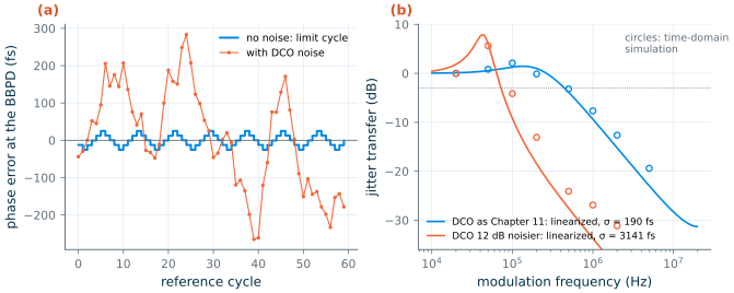
Eq. (15.11) explains the appeal. With σ = 190 fs the bang-bang detector’s equivalent floor is −123.2 dBc/Hz, against −84.3 dBc/Hz for the 43.5 ps TDC: in a low-jitter loop, one bit placed exactly at the edge resolves better than many bits spread across the period. The catch is fractional-N. A BBPD only works within a few σ of lock, so the predictable fractional phase (here 0.1 UI per cycle) must be removed before the detector, by a digital-to-time converter that delays the reference edge by the known amount. That combination is the basis of today’s low-jitter fractional-N digital PLLs [158].
15.6 Delay-locked loops
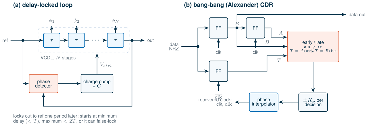
A delay-locked loop (DLL) aligns the output of a voltage-controlled delay line (VCDL) with its input one period later (Figure 15.7a). A phase detector compares the line’s input and output edges, a charge pump and capacitor (or a counter) integrate the error, and the integrated value sets the delay. There is no oscillator: the line only delays the reference, so a disturbance passes through once and is gone. Noise does not accumulate from cycle to cycle as it does in a VCO, and the loop, with a single integrator, is first-order and easy to stabilize [159, 11]. The price is that a DLL cannot synthesize a new frequency: its output frequency is its input’s, and the reference’s jitter goes straight through.
The common hazard is false lock. A phase detector cannot tell a delay of one period from a delay of two, or a delay stuck at its minimum from one that is still too short. A DLL therefore starts at its minimum delay, which must be shorter than one period, and its maximum delay must stay below two periods. The inverter line of Section 15.2 shows how hard that can be: its delay changes by a factor of 1.57 over supply and temperature, so a line that spans one period in the fastest corner spans 1.57 periods in the slowest, and the control range must cover that without reaching two.
DLLs supply the multi-phase clocks of time-interleaved converters and memory interfaces. In an ADPLL they offer a second way to normalize a TDC: a DLL that locks an N-stage line to the DCO period makes each stage exactly \(T_V/N\) in every corner, replacing the digital gain estimate of Section 15.2 by an analog loop.
15.7 Clock and data recovery
A serial data receiver gets no clock, only data. Clock and data recovery (CDR) extracts one from the transitions of the data and samples the data with it. Random non-return-to-zero (NRZ) data has a transition in only half its bit periods, and none during long runs of equal bits, so the phase detector must work with missing edges, and say nothing when there is no transition.
Two detectors dominate. The Hogge detector is linear: an XOR gate produces a pulse from each data transition to the next sampling clock edge, whose width grows with the phase error, and a second XOR produces a reference pulse of half a bit, so the difference of the two averages is proportional to the error [161]. The Alexander detector is bang-bang (Figure 15.7b): it samples the data at the centre of each bit and at the edge between bits. If a transition occurred, the edge sample equals either the bit before or the bit after, which tells whether the clock is early or late; with no transition it gives no output [160]. The bang-bang version is the norm at high data rates, because its decisions come from the same kind of flip-flops that sample the data.
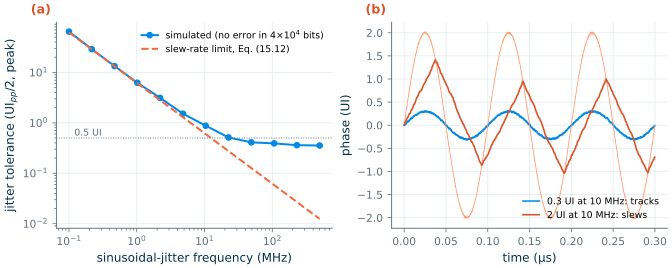
A CDR is specified by three jitter properties: jitter transfer, the low-pass response from input to recovered-clock jitter; jitter generation, the jitter it adds with clean data; and jitter tolerance, the largest sinusoidal input jitter, against its frequency, at which it still receives without errors. Slow input jitter is tracked; jitter beyond the loop bandwidth must fit in the eye. A bang-bang CDR adds a third regime, slewing: the recovered phase moves by a fixed step \(K_p\) per decision, at most \(D_T K_p\) per bit with a transition density \(D_T\) = 1/2, so a sinusoid of peak amplitude \(A\) (UI) at frequency \(f_{SJ}\) is tracked only while its slope stays below that:
\[A_{tol} \approx \frac{D_T\,K_p\,f_{bit}}{2\pi f_{SJ}}. \tag{15.12}\]Figure 15.8 shows a behavioural first-order bang-bang CDR at 10 Gb/s with \(K_p = 2^{-7}\) UI (7.81 mUI), random data and 0.01 UI rms of random jitter. Below a few megahertz the simulated tolerance follows Eq. (15.12) (median ratio 1.02; 6.42 UI against 6.22 UI at 1 MHz). Eq. (15.12) falls to half a UI at 12.4 MHz; above a few tens of megahertz the loop no longer follows and the tolerance flattens (0.358 UI, the median above 150 MHz), what is left of the half-UI eye after the random jitter and the loop’s own dither. A real CDR adds an integral path, as in Eq. (15.7), to track the frequency offset between transmitter and receiver crystals; it raises the low-frequency tolerance further [2].
Try it · The digital-PLL script
Every number in this chapter comes from
tools/figs/ch15_digital_pll.py:python3 tools/figs/ch15_digital_pll.pyredraws everything in under a minute (the ngspice delay lines are cached;--resimreruns them, about a minute each). Three experiments: (1) Halve the inverter widths (WN,WP) and runtdc --resim: does the delay change, and why does a smaller inverter not make a faster TDC when the load scales with it? (2) Force a wide loop withNUM_LOOP.update(alpha=2**-5, rho=2**-11)beforepart_pn()and compare the 1 MHz phase noise with Worked example 15.1. (3) ChangeFCWto 122.0 and to 122.25 and rerunpnwith the TDC dither off: where do the spurs go, and what happens to the in-band noise?
- An ADPLL counts phase in DCO cycles: a reference accumulator, an edge counter plus a TDC, a PI filter and a capacitor-bank DCO replace the PFD, charge pump, loop-filter capacitor (224 pF for a 200 kHz analog loop around the course VCO) and varactor.
- The TDC sets the in-band floor, (2π Δtres fDCO)²/(12 fref). One SG13G2 inverter delay, 43.5 ps (35.0–54.8 ps over supply and temperature), gives −84.3 dBc/Hz at 4.884 GHz, right at the course budget; a Vernier pair resolves 17.5 ps.
- DCO steps of 250 kHz (55.2 aF in the Chapter 11 tank) would add −98.9 dBc/Hz at 1 MHz; a second-order delta-sigma dither at 640 MHz makes them negligible.
- The type-II digital loop with α = 2−8, ρ = 2−17 (27.4 kHz) minimizes the integrated phase error, meets the 1 MHz specification with 8.9 dB of margin, and settles a channel step in 4.8 µs with gear shifting. Without dither, the TDC’s rounding makes fractional spurs (−67.5 dBc at 2 MHz from the LO).
- A bang-bang detector’s gain is √(2/π)/σ: its loop’s bandwidth depends on its jitter, and in a quiet loop its equivalent noise (−123.2 dBc/Hz) is far below a multi-bit inverter TDC’s.
- DLLs delay instead of oscillate, so their jitter does not accumulate, but they must avoid false lock; bang-bang CDRs track slow jitter up to their slew rate, DTKpfbit/(2πfSJ).
Further reading
- R. B. Staszewski and P. T. Balsara [154] on the phase-domain ADPLL, and the Bluetooth transmitter of Staszewski et al. [153], the first ADPLL in a commercial radio, with the DCO architecture in [152] and the TDC in [155].
- N. Da Dalt [157] on the nonlinear dynamics of bang-bang PLLs, and D. Tasca et al. [158] for a fractional-N bang-bang digital PLL with a digital-to-time converter.
- P. Dudek, S. Szczepański and J. V. Hatfield [156] on the Vernier delay-line TDC; J. G. Maneatis [159] on self-biased DLLs and PLLs.
- J. D. H. Alexander [160] and C. R. Hogge [161], the two short papers behind most CDR phase detectors.
- B. Razavi, Design of CMOS Phase-Locked Loops [11], and S. Palermo’s ECEN 620 notes [2], for digital PLLs, DLLs and CDRs in the context of the whole PLL family; F. M. Gardner [12] for sampled loops.