Chapter 7
On-Chip Passives
An RF circuit is only as good as its passive components. The inductors set the noise figure of the LNA and the phase noise of the VCO, capacitors and varactors tune them, transformers couple stages, and at millimetre waves the wires themselves become transmission lines. This chapter characterizes SG13G2's passives with ngspice and with electromagnetic simulation in Palace, and fits the inductor models that the rest of the course uses.
- Explain why every on-chip passive has a quality factor and a self-resonance, and calculate both from an equivalent circuit.
- Compare SG13G2’s MIM capacitor models and choose a capacitor size and feed for a given frequency.
- Estimate the inductance of a spiral with a closed-form expression, and name the mechanisms that limit its Q.
- Simulate a spiral inductor with Palace through IHP’s gds2palace flow, extract L(f), Q(f) and the self-resonance, and fit a π model to the result.
- Characterize a varactor, a switched capacitor, a transformer and an on-chip transmission line for the course radio.
Contents
7.1 Resistors and capacitors at RF
At low frequencies a capacitor is a capacitance and a resistor a resistance. At gigahertz frequencies every component also stores energy in the “wrong” field and loses some of it as heat. Two numbers describe how far a real component is from the ideal one: its quality factor and its self-resonance.
The quality factor Q of a reactive component compares the energy it stores with the energy it loses. With an impedance \(Z = R + jX\),
\[Q = \frac{\lvert X\rvert}{R} = 2\pi\,\frac{\text{peak energy stored}}{\text{energy lost per cycle}}, \tag{7.1}\]so a series resistance \(R\) gives a capacitor and an inductor
\[Q_C = \frac{1}{\omega R C}, \qquad Q_L = \frac{\omega L}{R}. \tag{7.2}\]A capacitor’s Q falls with frequency, an inductor’s rises (until other losses take over, Section 7.3). The parasitic inductance \(L_p\) of a capacitor, or the parasitic capacitance \(C_p\) of an inductor, makes the component resonate at its self-resonance frequency (SRF)
\[f_{SRF} = \frac{1}{2\pi\sqrt{L C_p}} \quad\text{or}\quad \frac{1}{2\pi\sqrt{L_p C}}, \tag{7.3}\]above which a capacitor behaves as an inductor and an inductor as a capacitor. A component is used well below its SRF, where its effective value is still close to the nominal one. In a resonant circuit the losses of all components add: the Q of an LC tank is \(1/Q_{tank} = 1/Q_L + 1/Q_C\), so the worse of the two sets the tank Q, and with it the noise figure of an LNA or the phase noise of an oscillator (Chapter 11).
Resistors in SG13G2 are polysilicon (rsil, rppd, rhigh) on the field oxide. At RF the problem is their capacitance to the substrate, distributed along the resistor: a resistor of value \(R\) and total substrate capacitance \(C_{sub}\) behaves as a distributed RC line with a corner near \(1/(2\pi R C_{sub})\). In RF paths, resistors are therefore kept short and wide (a small area means a small \(C_{sub}\)), and bias resistors that should block RF are made large on purpose [10, 7]. This chapter does not simulate them further.
MIM capacitors: cap_cmim and cap_rfcmim
SG13G2’s MIM capacitor is a thin, high-permittivity dielectric between a Metal5 bottom plate and a thin top plate that vias connect to TopMetal1 (Figure 7.1a) [191]. Its capacitance has an area and an edge term,
\[C = C_A\,W L + C_P\cdot 2(W + L), \qquad C_A = 1.5\ \mathrm{fF/\mu m^2},\ C_P = 40\ \mathrm{aF/\mu m}, \tag{7.4}\]with the values of the PDK’s typical corner. The PDK offers two models of the same device. cap_cmim is the capacitance of Eq. (7.4) with a fixed 55 mΩ in series, good for analog work. cap_rfcmim is the RF model of Figure 7.1b: a plate and feed inductance \(L_{mim} + L_{feed}\), the plate resistance \(R_{mim}\) (which includes the resistance of the feed line, \(0.96\ \Omega\cdot\mu\mathrm{m}/w_{feed}\)), a skin-effect branch, and the bottom plate’s coupling to the substrate through \(C_{ox}\) and \(C_{sub}\parallel R_{sub}\). Its element values are polynomials in \(W\), \(L\) and the feed width \(w_{feed}\), fitted by IHP to measurements of plates from 7 to 75 µm.
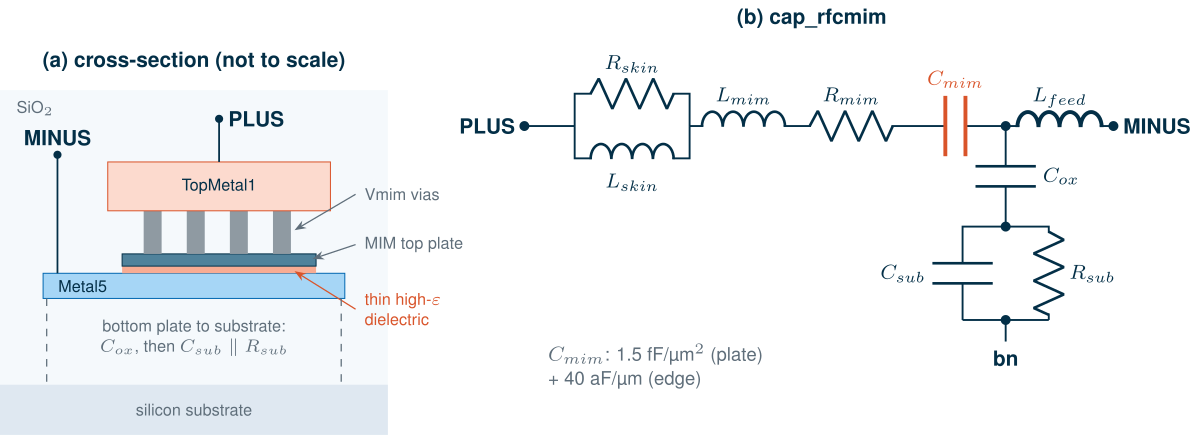
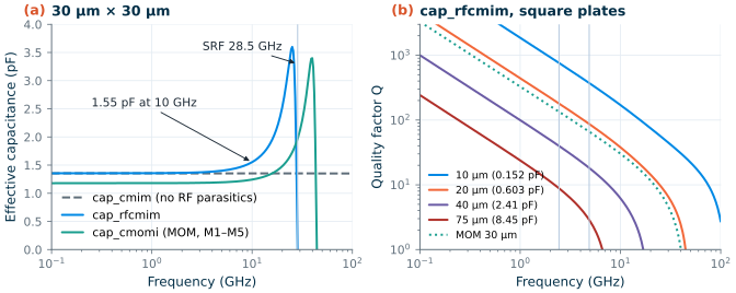
Figure 7.2 compares the two models in an ngspice S-parameter analysis. A 30 µm × 30 µm plate has 1.35 pF at low frequency in both. With cap_rfcmim the effective capacitance \(\mathrm{Im}(Y)/\omega\) rises to 1.55 pF at 10 GHz, as the series inductance resonates with the capacitance at 28.5 GHz; cap_cmim stays at 1.35 pF for ever. The Q is where the two models disagree most: at the VCO frequency of 4.88 GHz, cap_cmim promises Q = 438, cap_rfcmim gives 35.6.
Worked example 7.1 · The Q of a MIM capacitor in the VCO tank
A 30 µm × 30 µm cap_rfcmim with the default 2 µm feed. From the model’s equations, \(R_{mim}\) = 0.628 Ω, of which 0.481 Ω is the feed term \(0.96/w_{feed}\). At 4.88 GHz the skin branch adds 0.0256 Ω (its inductance nearly shorts its resistance), so \(R \approx\) 0.654 Ω. The reactance of 1.35 pF is \(1/\omega C\) = 24.1 Ω, and Eq. (7.2) gives
\[Q_C = \frac{X_C}{R} = \frac{24.1}{0.654} \approx 36.8,\]close to the simulated 35.6 (the substrate network and the rising effective capacitance lower it a little). Nearly three quarters of the resistance is the narrow feed. With \(w_{feed}\) = 10 µm, \(R\) drops to 0.269 Ω and \(Q_C \approx\) 89.4 by hand, 87.3 in simulation. The series inductance, 18.3 pH, puts the hand-calculated SRF at 32 GHz (simulated: 28.5 GHz).
The plate size matters as much as the feed (Table 7.1). Since \(R_{mim}\) hardly depends on the area while \(X_C\) falls as \(1/(WL)\), the Q of Eq. (7.2) falls roughly in proportion to the area: a 10 µm plate has Q = 373 at 4.88 GHz, a 75 µm plate only 2.88, and the 75 µm plate self-resonates at 7.94 GHz. A large RF capacitance is better built from several smaller plates in parallel, each with a wide feed.
Table 7.1. Square cap_rfcmim capacitors (2 µm feed) and a MOM capacitor: capacitance, Q at the course radio's two frequencies and self-resonance (ngspice, typical corner).
| Capacitor | C at low f | Q at 2.44 GHz | Q at 4.88 GHz | SRF |
|---|---|---|---|---|
| cap_rfcmim 10 µm × 10 µm | 0.152 pF | 760 | 373 | above 100 GHz |
| cap_rfcmim 20 µm × 20 µm | 0.603 pF | 180 | 86.9 | 48.2 GHz |
| cap_rfcmim 30 µm × 30 µm | 1.35 pF | 75.2 | 35.6 | 28.5 GHz |
| cap_rfcmim 30 µm × 30 µm, 10 µm feed | 1.35 pF | 191 | 87.3 | 33.3 GHz |
| cap_rfcmim 40 µm × 40 µm | 2.41 pF | 39.8 | 18.2 | 19.2 GHz |
| cap_rfcmim 75 µm × 75 µm | 8.45 pF | 8.83 | 2.88 | 7.94 GHz |
| cap_cmomi 30 µm × 30 µm (MOM) | 1.18 pF | 134 | 66.1 | 44.2 GHz |
MOM capacitors
A MOM capacitor needs no special dielectric: interdigitated fingers on several metal layers, connected alternately to the two terminals, use the lateral field between the fingers, which grows as the metal pitch shrinks [102]. SG13G2 has two: cap_cmomi (interdigitated, with an RF model fitted to about 50 GHz) and cap_cmomf (fringe fingers, low-frequency model only). Both are Verilog-A models loaded into ngspice through OSDI. With Metal1 to Metal5, cap_cmomi gives 1.31 fF/µm², close to the MIM’s 1.5, with Q = 66.1 at 4.88 GHz and an SRF of 44.2 GHz for a 30 µm square (Figure 7.2). MOM capacitors are symmetric and match well; MIM capacitors have a smaller bottom-plate parasitic relative to their value and sit above the active area, so the two are often used side by side.
What this means for your design
In a 2.4 GHz matching network or a 4.9 GHz tank, a MIM capacitor of a few hundred femtofarads to about 1 pF has a Q of 50–400 and is rarely the weakest element; the inductor is. Large capacitors (DC blocks of several picofarads) have a low Q and an SRF that can fall into the band: split them into smaller plates, use wide feeds, and always simulate with cap_rfcmim, not cap_cmim.
7.2 Spiral inductors
An inductor stores energy in its magnetic field. On a chip there is no room for a coil with a core, so inductors are planar spirals in the thickest, highest metals, far from the lossy substrate. SG13G2 has two thick top metals for this: TopMetal2, 3 µm thick with a sheet resistance of 11 mΩ/□, and TopMetal1, 2 µm thick (18 mΩ/□), both about 11 µm and 6 µm above the silicon [191, 198].
Figure 7.3 shows the four inductors this chapter characterizes. They are symmetric octagonal spirals, the shape of the PDK’s inductor2 cell: each turn is split into a left and a right half, and adjacent turns swap sides at crossings at the top and the bottom, where one track dips to TopMetal1 through TopVia2. Both terminals are at the bottom of the outer turn, so the spiral is symmetric about its vertical axis, which suits differential circuits such as the VCO. A spiral is described by its number of turns \(N\), its outer diameter \(d_{out}\) (flat to flat), the track width \(w\) and the spacing \(s\) (2.1 µm here, the PDK default); the inner diameter is \(d_{in} = d_{out} - 2Nw - 2(N-1)s\).
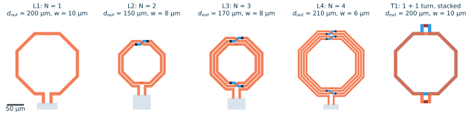
tools/em/ch07_inductors/ch07_geom.py, with the Metal1 ground frame used in the EM simulation (not shown). Same scale in all panels.How much inductance?
Wheeler’s formula for solenoids [93], adapted to planar spirals by Mohan, Hershenson, Boyd and Lee [94], estimates the inductance from the geometry alone. With the average diameter \(d_{avg} = (d_{out} + d_{in})/2\) and the fill ratio \(\rho = (d_{out} - d_{in})/(d_{out} + d_{in})\), the modified Wheeler formula is
Key equation · Inductance of a planar spiral
\[L \approx K_1\,\mu_0\,\frac{N^2 d_{avg}}{1 + K_2\,\rho}, \qquad K_1 = 2.25,\ K_2 = 3.55\ \text{(octagon)}. \tag{7.5}\]The inductance grows with the square of the number of turns and in proportion to the size. A large fill ratio (turns that reach far towards the centre) adds turns whose small loops add little flux, hence the denominator.
The same paper gives a second expression from the current-sheet approximation, which treats the turns as a uniform sheet of current,
\[L \approx \frac{\mu_0 N^2 d_{avg}\,c_1}{2}\left[\ln\frac{c_2}{\rho} + c_3\,\rho + c_4\,\rho^2\right], \qquad (c_1, c_2, c_3, c_4) = (1.07,\ 2.29,\ 0,\ 0.19), \tag{7.6}\]and both are quoted as accurate to a few per cent for spirals that are not too sparse. Neither includes the feed lines or the crossings.
Worked example 7.2 · Sizing a 1 nH spiral
Take \(N\) = 2, \(w\) = 8 µm, \(s\) = 2.1 µm and \(d_{out}\) = 150 µm (inductor L2). Then \(d_{in}\) = 150 − 32 − 4.2 = 114 µm, \(d_{avg}\) = 132 µm and \(\rho\) = 0.137. Eq. (7.5):
\[L = 2.25 \times 4\pi\times10^{-7} \times \frac{4 \times 132\ \mu\mathrm{m}}{1 + 3.55 \times 0.137} = 1.00\ \mathrm{nH},\]and Eq. (7.6) gives 1.00 nH. The track is 924 µm long (two turns and two 25 µm feeds), so its DC resistance on TopMetal2 is \(R_{DC} = l\,R_\square/w\) = 1.27 Ω. The electromagnetic simulation of Section 7.4 gives 0.9 nH at 1 GHz: the closed-form estimates are about 10 % high for this symmetric spiral.
Where the energy goes
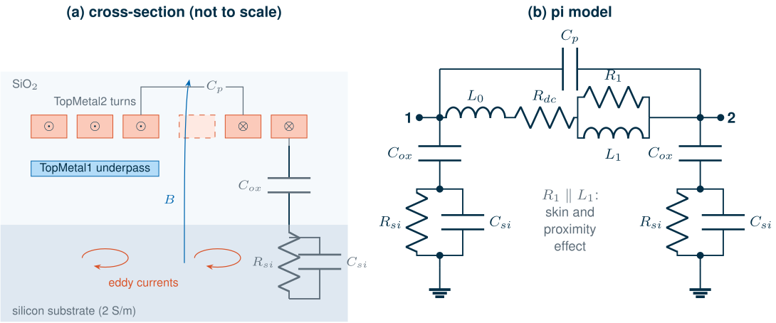
Three mechanisms limit the Q of a spiral (Figure 7.4a) [95, 96, 99].
Resistance of the metal. At DC the resistance is \(R_{DC} = l/(\sigma w t)\). At high frequencies the current crowds towards the surfaces of a conductor, within the skin depth \(\delta\). For a strip of thickness \(t\) that carries current on both faces, the one-dimensional solution gives [14, 7]
\[\delta = \frac{1}{\sqrt{\pi f \mu_0 \sigma}}, \qquad \frac{R(f)}{R_{DC}} = \frac{t}{2\delta}\cdot\frac{\sinh(t/\delta) + \sin(t/\delta)}{\cosh(t/\delta) - \cos(t/\delta)} \;\to\; \frac{t}{2\delta} \quad (\delta \ll t). \tag{7.7}\]For TopMetal2 (\(\sigma\) = 3.03 × 10⁷ S/m), \(\delta\) equals the 3 µm thickness at 0.929 GHz and is 1.85 µm at 2.44 GHz, 1.31 µm at 4.88 GHz and 0.409 µm at 50 GHz; Eq. (7.7) raises the resistance by a factor of 1.14 at 4.88 GHz and 1.51 at 10 GHz. In a spiral the proximity effect adds to this: the magnetic field of the neighbouring turns crosses each turn and induces eddy currents in it, pushing the current towards one edge, so the resistance of a multi-turn spiral rises faster than Eq. (7.7) predicts [97]. The field is strongest at the centre, which is why the innermost turns, which add little inductance, are left out: a hollow spiral (small \(\rho\)) has a higher Q.
Capacitive substrate loss. The voltage on the spiral drives a displacement current through the oxide capacitance \(C_{ox}\) into the silicon, which conducts (2 S/m, about 50 Ω cm, in SG13G2) and dissipates it in \(R_{si}\). This loss grows with frequency and with the area of the spiral.
Magnetic substrate loss. The alternating magnetic field reaches into the silicon and induces eddy currents there that flow opposite to the spiral’s current. They lower the inductance slightly and dissipate power. Both substrate losses are why inductors are drawn in the top metals, with no other metal, active area or fill underneath (the PDK cell blocks them).
The π model
A spiral used as a two-port is described by the π model of Figure 7.4b [95, 98]. The series branch carries the inductance and the metal loss; in the classical model it is a constant \(L_s\) and \(R_s\), which fits only a narrow band, because \(R_s\) rises with frequency. Following Cao et al. [98], we split the inductance into \(L_0\) and \(L_1\) and put a resistor \(R_1\) across \(L_1\): at low frequencies \(L_1\) shorts \(R_1\) and the branch is \(L_0 + L_1\) with \(R_{DC}\); at high frequencies the current moves into \(R_1\), the resistance rises and the inductance falls a little, as in the real spiral. \(C_p\) models the capacitance between the turns and between the underpass and the turns; at each port, \(C_{ox}\) couples to the substrate, modelled as \(R_{si} \parallel C_{si}\). All eight values are frequency-independent, so the model works in every SPICE analysis, transient included.
7.3 Quality factor and self-resonance
A spiral is a two-port, and its Q depends on how it is connected. With port 2 grounded (a single-ended inductor, as in an LNA’s source degeneration or a matching network), the impedance seen at port 1 is \(1/Y_{11}\); driven between its two ports with the ground floating (differential, as in a VCO tank), it is \(Z_d = Z_{11} + Z_{22} - Z_{12} - Z_{21}\). In both cases
\[L = \frac{\mathrm{Im}\,Z}{\omega}, \qquad Q = \frac{\mathrm{Im}\,Z}{\mathrm{Re}\,Z}, \qquad Z = \frac{1}{Y_{11}}\ \text{or}\ Z_d, \tag{7.8}\]and the SRF is where \(\mathrm{Im}\,Z\) crosses zero. (A definition based on stored energies differs from Eq. (7.8) near the SRF, where Eq. (7.8) falls to zero; for an inductor used well below its SRF the two agree.)
The π model shows how Q varies with frequency. Neglecting the skin effect, Yue and Wong [95] write the single-ended Q as a product of three factors,
\[Q = \underbrace{\frac{\omega L_s}{R_s}}_{\text{metal loss}} \cdot \underbrace{\frac{R_p}{R_p + \left[(\omega L_s/R_s)^2 + 1\right]R_s}}_{\text{substrate loss}} \cdot \underbrace{\left[1 - \frac{R_s^2\,(C_s + C_p)}{L_s} - \omega^2 L_s\,(C_s + C_p)\right]}_{\text{self-resonance}}, \tag{7.9}\]where \(R_p\) and \(C_s\) are the parallel equivalents of the shunt branch (\(C_{ox}\) in series with \(R_{si} \parallel C_{si}\)) at port 1. At low frequencies only the first factor matters and Q rises in proportion to \(f\) (less as the skin effect raises \(R_s\)). As the frequency rises, the substrate factor falls, and the last factor drives Q to zero at the SRF. Q therefore peaks somewhere below the SRF, and a good inductor for a given frequency is one whose peak Q falls near that frequency.
Differential drive raises Q. Driven differentially, the two shunt branches are in series between the terminals, each seeing half the voltage swing, so the substrate dissipates less for the same stored energy, and the SRF rises because the shunt capacitances appear in series [100]. Section 7.4 quantifies the gain for our spirals.
7.4 Electromagnetic simulation of an SG13G2 inductor
Closed-form expressions give the inductance within a few per cent, but not the Q or the SRF: those depend on the current distribution in the metal and on the fields in the substrate, which only an electromagnetic (EM) simulation captures. Chapter 2 introduced the two open-source EM solvers in IIC-OSIC-TOOLS: openEMS, a finite-difference time-domain solver, and Palace, a finite-element frequency-domain solver [196, 197]. IHP provides flows for both that read a GDSII layout and an XML description of the SG13G2 stack-up [198, 206]. We use Palace through gds2palace, which IHP’s own inductor-synthesis examples use.
The flow
- Layout.
tools/em/ch07_inductors/ch07_geom.pydraws each spiral with gdspy on the SG13G2 layer numbers, surrounds it with a 20 µm wide Metal1 ground frame at a distance of half the diameter (at least 60 µm), brings Metal1 under the two feeds, and draws each port as a thin box on layers 201 and 202. - Stack-up. IHP’s
SG13G2_200um.xml: a 200 µm thick chip, a 2 S/m substrate under a 3.75 µm, 5 S/m EPI layer, 15.7 µm of oxide (\(\varepsilon_r\) = 4.1) with the metals at their real heights, thicknesses and conductivities (TopMetal2: 3.03 × 10⁷ S/m; TopMetal1: 2.78 × 10⁷ S/m), a passivation layer and air above. - Model. gds2palace merges the polygons, models each metal as an impedance sheet that accounts for its thickness and conductivity, meshes the volume with gmsh (5 µm on the conductors, at most 70 µm elsewhere), and turns the port boxes into vertical lumped ports of 50 Ω from Metal1 up to the feed.
- Solve. Palace solves Maxwell’s equations with second-order elements at a few frequencies chosen by its adaptive sweep and builds a reduced-order model that interpolates the S-parameters at all others, from 0.01 GHz to 20–50 GHz (100 GHz for the lines). Because the spirals are symmetric, only port 1 is excited, and \(S_{22} = S_{11}\), \(S_{12} = S_{21}\).
- Post-process.
tools/em/ch07_inductors/ch07_palace.pywrites a Touchstone file, andtools/figs/ch07_passives.pyreads it withrfic.rf.read_snp, computes Eq. (7.8) and fits the π model.
We first ran IHP’s own reference inductor, L_2n0, with these settings to calibrate the cost: its mesh gives 246066 unknowns (second-order elements), each frequency sample is one sparse solve that converges in 25–32 GMRES iterations, and the adaptive sweep needed 8 samples per excitation for 0.01–50 GHz. On four cores of a laptop shared with other jobs that is several minutes per sample; exciting one port instead of two halves it. With one excitation, our spirals then took 9 to 21 minutes each. Accuracy is checked against closed-form estimates below and against an independent commercial-solver result at the end of this section.
Results
Figure 7.5 shows the inductance and Q of the four spirals, and Table 7.2 collects the numbers. The inductance is flat at low frequencies, then rises towards the SRF, where the parasitic capacitance resonates with it. L1, a single 200 µm turn, has 0.439 nH; L2, the 1 nH spiral of Worked example 7.2, has 0.9 nH; L3 1.92 nH and L4 4.73 nH. The modified Wheeler formula is within 11 % of the EM values, and the current-sheet expression within 11 %.
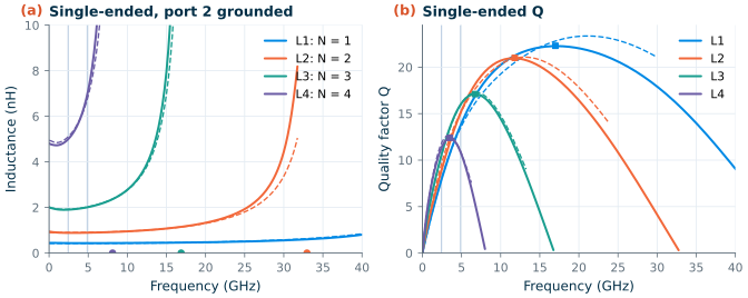
The Q curves follow Eq. (7.9). At 2.44 GHz, the band of the course radio, the single-ended Q is 7.91, 8.91, 10.6 and 11.3 from L1 to L4; at 4.88 GHz 13.7, 15.1, 16 and 10.8. The peak Q falls from 22.3 (L1, at 17 GHz) to 12.4 (L4, at 3.5 GHz), and the SRF from above 50 GHz (L1) to 8.12 GHz.
Table 7.2. The inductor family: geometry, closed-form estimates and EM results (Palace, single-ended unless marked; L at 1 GHz).
| L1 | L2 | L3 | L4 | |
|---|---|---|---|---|
| N, dout, w | 1, 200 µm, 10 µm | 2, 150 µm, 8 µm | 3, 170 µm, 8 µm | 4, 210 µm, 6 µm |
| L, Eq. (7.5) / Eq. (7.6) | 0.453 / 0.482 nH | 1.00 / 1.00 nH | 2.12 / 2.1 nH | 5.09 / 5.05 nH |
| L (EM) | 0.439 nH | 0.9 nH | 1.92 nH | 4.73 nH |
| R at 0.01 GHz (EM) / RDC by hand | 0.724 / 0.748 Ω | 1.14 / 1.27 Ω | 1.74 / 2.01 Ω | 3.41 / 4.46 Ω |
| Q at 2.44 GHz | 7.91 | 8.91 | 10.6 | 11.3 |
| Q at 4.88 GHz (differential) | 13.7 (14) | 15.1 (15.6) | 16 (17.7) | 10.8 (15.6) |
| Peak Q, at | 22.3, 17 GHz | 21, 11.8 GHz | 17.1, 6.75 GHz | 12.4, 3.5 GHz |
| SRF (differential) | above 50 GHz | 33 (39.6) GHz | 16.9 (18.7) GHz | 8.12 (8.65) GHz |
The resistance at the lowest simulated frequency is 10–25 % below the hand value \(l R_\square/w\). We attribute this to the way gds2palace represents a metal: by its surfaces, each with the conductivity and thickness of the layer, which is accurate when the skin depth is smaller than the thickness (above about 0.929 GHz on TopMetal2) but only approximate at DC, where the current fills the whole cross-section. Below 1 GHz the EM Q of our spirals is therefore somewhat optimistic; at the frequencies of the course radio it is not affected.
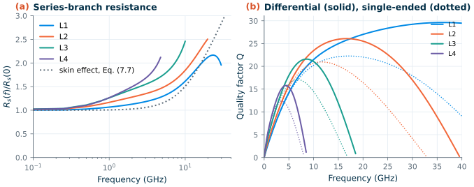
Figure 7.6a shows the resistance of the series branch, \(\mathrm{Re}(-1/Y_{12})\), relative to its low-frequency value. Every spiral rises faster than the skin effect of an isolated strip, Eq. (7.7), and the more turns, the faster: at 4.88 GHz Eq. (7.7) predicts a factor of 1.14, while the EM resistance has risen by 1.28 (L1), 1.47 (L2), 1.72 (L3) and 2.17 (L4). That is the proximity effect of Section 7.2, and it is why the Q of the larger spirals peaks at a lower value. Figure 7.6b compares the differential Q with the single-ended one. As Section 7.3 predicted, differential drive raises the peak Q and moves it and the SRF to higher frequencies; the gain is largest for the large spirals, whose substrate loss matters most: at 4.88 GHz, L4 has a differential Q of 15.6 against 10.8 single-ended, L2 15.6 against 15.1.
The π model for the rest of the course
For each spiral, tools/figs/ch07_passives.py fits the eight values of the π model of Figure 7.4b to the EM Y-parameters, from the lowest simulated frequency to 0.8 times the SRF (least squares on the series impedance \(-1/Y_{12}\) and the shunt admittance \(Y_{11} + Y_{12}\), with relative errors). Table 7.3 lists the result, and the dashed lines of Figure 7.5 show how well it reproduces L and Q: the series impedance is matched to 0.9–3.3 % rms, and the Q at 2.44 and 4.88 GHz to within 8 %.
Table 7.3. Fitted π-model values (Figure 7.4b) and the upper frequency of the fit.
| L0 | L1 | Rdc | R1 | Cp | Cox | Rsi | Csi | fit to | |
|---|---|---|---|---|---|---|---|---|---|
| L1 | 410 pH | 14.1 pH | 0.755 Ω | 0.887 Ω | 0.5 fF | 33.7 fF | 1020 Ω | 45.5 fF | 30 GHz |
| L2 | 868 pH | 26.8 pH | 1.26 Ω | 1.06 Ω | 8.19 fF | 30.3 fF | 1420 Ω | 33.8 fF | 24 GHz |
| L3 | 1850 pH | 130 pH | 1.75 Ω | 1.03 Ω | 26.2 fF | 40.4 fF | 1540 Ω | 34.9 fF | 13.5 GHz |
| L4 | 4670 pH | 278 pH | 3.42 Ω | 1.35 Ω | 47.1 fF | 52 fF | 1470 Ω | 39.3 fF | 6.49 GHz |
Later chapters need inductors of other values: the LNA’s gate and source inductors, the VCO’s tank, the matching networks of the PA. The module tools/figs/_ch07_inductor.py serves the fitted family to them. It interpolates each π-model value in log–log against the DC inductance \(L_0 + L_1\), so a 2 nH inductor gets values between those of L2 and L3, and returns netlist lines that work in ngspice and in Xyce alike:
import sys; sys.path.insert(0, "tools/figs")
from _ch07_inductor import inductor_lines
lines = inductor_lines("g", "in", "gate", 2.0)              # 2.0 nH between nodes in and gate
lines = inductor_lines("t", "outp", "outn", 1.0, ct="vdd")  # differential, centre tap to vdd
* g: SG13G2 octagonal spiral, EM-fitted pi model (Chapter 7), Ldc = 2 nH, valid to 13 GHz
Lg0 in g_a 0.000
Rgdc g_a g_b 1.77
Rg1 g_b gate 1.03
Lg1 g_b gate 0.000
Cgp in gate 0.000
Cgox1 in g_s1 0.000
Rgsi1 g_s1 0 1540
Cgsi1 g_s1 0 0.000
...
The model is valid for inductances from 0.424 to 4.94 nH and from DC to the fit limit of Table 7.3 (interpolated in the same way); outside that range the function refuses to extrapolate. The Touchstone files of the four spirals are in tools/em/ch07_inductors/ for simulators that can use S-parameters directly.
Common pitfall · Trusting an EM result you have not checked
An EM solver answers the question you asked, which is not always the one you meant. Our models have no metal fill, no guard ring with substrate contacts (the Metal1 frame is the only return path), lumped ports a few micrometres tall whose inductance is included in the result, and a 5 µm mesh that resolves the current crowding across an 8 µm track only coarsely. Check every new structure with a closed-form estimate (Eqs. (7.5)–(7.7)), with a finer mesh, and, when the result matters, with a second solver: IHP provides the same inductors for openEMS.
An independent check: the 4 nH inductor of an SG13G2 PLL
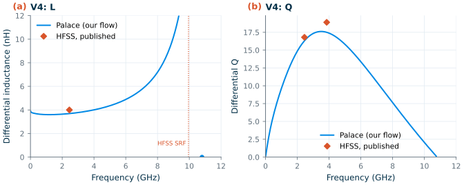
Our flow has so far only been checked against closed-form estimates. An independent check comes from a taped-out SG13G2 design: the 2.4 GHz LC-VCO fractional-N PLL of Thiriloganathan et al. [106, 207], whose tank inductor was characterized with a commercial finite-element solver (Ansys HFSS). It has the topology of our family, a symmetric octagon on TopMetal2 with TopMetal1 crossings and the feeds on the outer turn, with 3 turns, 30 µm wide tracks spaced 14 µm, an outer radius of 218 µm to the centre of the outer track (\(d_{out}\) = 466 µm) and 105 µm long feeds. HFSS gives \(L_{diff}\) = 4.00 nH and \(Q_{diff}\) = 16.8 at 2.45 GHz, a peak Q of 18.9 near 3.85 GHz and an SRF of 9.95 GHz. We redrew the same parameters with our own script (V4 in ch07_geom.py; the crossings and the Metal1 frame, where their layout has a substrate-contact ring, are ours) and simulated it with the same flow (8 µm mesh on the 30 µm tracks, 39 minutes).
Figure 7.7 compares the two. At 2.45 GHz Palace gives \(L_{diff}\) = 3.69 nH (−8 % from HFSS) and \(Q_{diff}\) = 16.3 (−3 %); the peak differential Q is 17.6 at 3.5 GHz and the differential SRF 10.8 GHz (+8 %). The Q at the operating frequency, the number that sets the VCO’s phase noise, agrees within a few per cent; the inductance is lower and the SRF higher by similar amounts, which points to the parts of the two models that differ: the crossings, the ports and their reference planes, and the return path. (Interestingly, the modified Wheeler formula gives 4.02 nH, closer to HFSS than to our result, while for our family it overestimates Palace by a similar margin.) The lesson is the one of the pitfall above: a few per cent in L and SRF is the accuracy to expect of an EM result, so a tank needs tuning range to absorb it. The π model fitted to this spiral (to 4 GHz) is available as inductor_lines(..., model="V4") for the case study of this VCO later in the course.
7.5 Transformers and baluns
Two spirals close to each other share magnetic flux: the current in one induces a voltage in the other. With self-inductances \(L_1\), \(L_2\) and mutual inductance \(M\), the coupling coefficient
\[k = \frac{M}{\sqrt{L_1 L_2}}, \qquad \begin{bmatrix} V_1 \\ V_2 \end{bmatrix} = j\omega \begin{bmatrix} L_1 & M \\ M & L_2 \end{bmatrix} \begin{bmatrix} I_1 \\ I_2 \end{bmatrix} \tag{7.10}\]measures how much of the flux of one winding links the other, from 0 to 1 for an ideal transformer. On chip, transformers couple the stages of an amplifier without DC connection, combine the outputs of PA cells, and as baluns convert a single-ended signal into a differential one [101]. The windings are either interleaved in the same metal layer, side by side, or stacked on top of each other in two metal layers, which gives a larger \(k\) for the same area, at the cost of a larger capacitance between the windings.
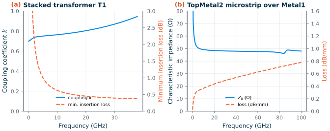
Our transformer T1 (Figure 7.3) is the simplest stacked one: a single 200 µm octagonal turn on TopMetal2 over an identical turn on TopMetal1, 2.8 µm below, with the feeds of the primary at the bottom and of the secondary at the top. Each winding is driven differentially by an in-plane port across its feed gap. From the EM Z-parameters, \(L_1\) = 0.437 nH, \(L_2\) = 0.441 nH and k = 0.72 at 1 GHz (Figure 7.9a); TopMetal2 is thicker than TopMetal1, so the primary’s Q is the higher of the two at 4.88 GHz: 13.4 against 9.64. The minimum insertion loss, \(-10\log_{10}G_{max}\) with both sides conjugately matched, is 1.78 dB at 2.44 GHz, 1.01 dB at 4.88 GHz and falls to a minimum of 0.372 dB near 38 GHz, below the windings’ self-resonance at 42.2 GHz, which is why such transformers are popular at millimetre waves (Chapter 17); at 2.4 GHz, a single turn’s 0.437 nH is too small for most uses and multi-turn windings are needed.
7.6 Varactors and switched capacitors
An LC oscillator is tuned by changing its capacitance: continuously with a varactor, in steps with switched capacitors. The course VCO must cover 4.80–4.97 GHz plus a margin for process and temperature (Chapter 11).
The accumulation-mode MOS varactor
A MOS capacitor whose gate is an n+ electrode over an n-well has no source of holes, so it never inverts. With the gate positive with respect to the well, electrons accumulate under the gate and the capacitance is the full oxide capacitance \(C_{ox}WL\); with the gate negative, the surface depletes and a depletion capacitance appears in series, which lowers the total. (Chapter 4 of The Art of Analog IC Design reviews accumulation, depletion and inversion in a MOS capacitor.) This accumulation-mode varactor has a monotonic, steep C–V characteristic and a good Q, because the electrons that carry the AC current are majority carriers that respond at any frequency [103, 104]. SG13G2’s sg13_hv_svaricap is such a device, built with the 3.3 V gate oxide: two gates G1 and G2 share one n-well W, so it is naturally a differential capacitor between G1 and G2, tuned by the well voltage. Its model (the MOSVAR compact model) includes the well and substrate parasitics.
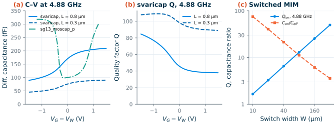
Figure 7.8a shows the differential capacitance between G1 and G2 at 4.88 GHz against \(V_G - V_W\), for \(W\) = 9.74 µm and 10 fingers, at the two ends of the allowed gate length. With \(L\) = 0.8 µm the capacitance tunes from 89.6 to 209 fF over ±1.5 V, a tuning ratio of 2.34 (2.17 over ±1.2 V), and the Q at 4.88 GHz is between 37.9 and 84.6. With \(L\) = 0.3 µm the ratio drops to 1.99, because the overlap and fringe capacitances, which do not tune, are a larger part of a short device, but the Q rises to at least 89, because the AC current crosses a shorter, less resistive path under the gate. Q is lowest in accumulation (Figure 7.8b), where the capacitance is largest and \(Q = 1/(\omega R_s C)\) smallest for a given series resistance \(R_s\).
For comparison, sg13_moscap_p is a thin-oxide PMOS with its source, drain and n-well tied together (a “B = D = S” MOS capacitor). Its C–V curve in Figure 7.8a is U-shaped: accumulation at positive voltage, depletion near zero (minimum at -0.1 V) and inversion at negative voltage, when the p+ source and drain supply holes. A non-monotonic C–V makes the oscillator’s tuning gain change sign, which is why B = D = S capacitors are not used as varactors [104]. (The sg13_moscap model has no series resistance, so its Q is not meaningful; it is meant for decoupling.)
Switched capacitors
A varactor large enough to cover the whole tuning range would give the VCO a large gain \(K_{VCO}\) and turn noise on the control voltage into phase noise. Oscillators therefore tune coarsely with a bank of switched capacitors and finely with a small varactor. A switched unit is two MIM capacitors with an NMOS switch between their bottom plates (biased through large resistors). On, the switch adds its resistance \(R_{on}\) in series with \(C_{on} \approx C/2\); off, its small capacitance \(C_{sw}\) in series leaves \(C_{off} \approx C_{sw}\) (for \(C \gg C_{sw}\)). Since \(R_{on} \propto 1/W\) and \(C_{sw} \propto W\),
\[Q_{on} = \frac{1}{\omega R_{on} C_{on}}, \qquad Q_{on}\cdot\frac{C_{on}}{C_{off}} \approx \frac{1}{\omega R_{on} C_{sw}}, \tag{7.11}\]and the product on the right is a property of the process, independent of the width: a wider switch buys Q with tuning ratio. Figure 7.8c shows this for two 20 µm × 20 µm cap_cmim plates and a minimum-length sg13_lv_nmos switch (rfmode = 1). From 10 to 320 µm, \(Q_{on}\) at 4.88 GHz rises from 1.65 to 49.7 while \(C_{on}/C_{off}\) falls from 75.1 to 3.58; their product stays between 124 and 178 (it creeps up because at large widths \(C_{sw}\) is no longer small against \(C\)).
7.7 On-chip transmission lines
At 2.4 GHz a wire on chip is a lumped element: the wavelength on a TopMetal2 line is 5.61 cm. At 50 GHz it is 3.1 mm, and an interconnect of a few hundred micrometres is a sizeable fraction of a wavelength: it must be designed as a transmission line (Chapter 3). The usual on-chip line is a microstrip: a TopMetal2 strip over a Metal1 ground plane, 9.77 µm below. The ground plane shields the lossy substrate, so the loss is mostly in the metal, and the field is mostly in the oxide.
The Hammerstad–Jensen formulas [105] for a strip of width \(w\) over a ground at height \(h\) in a dielectric of \(\varepsilon_r\) = 4.1 predict 50 Ω for \(w \approx\) 16.8 µm (and 51.3 Ω, \(\varepsilon_{eff}\) = 3.13, for 16 µm; they assume air above the strip, while ours is buried 1.5 µm deep in oxide); we simulated a 16 µm strip over an 80 µm wide Metal1 ground, in two lengths (300 and 900 µm), with Palace (stack-up without the substrate, as in IHP’s line example). The ports of an EM simulation add their own parasitics; comparing two lines removes them. With the transmission (ABCD) matrices \(\mathbf{T}_{300}\) and \(\mathbf{T}_{900}\) of the two simulations,
\[\mathbf{T}_{900}\,\mathbf{T}_{300}^{-1} = \mathbf{P}\,\mathbf{T}_{line}(600\ \mu\mathrm{m})\,\mathbf{P}^{-1}, \qquad \text{eigenvalues } e^{\pm\gamma\cdot 600\ \mu\mathrm{m}}, \quad \gamma = \alpha + j\beta, \tag{7.12}\]where \(\mathbf{P}\) is the matrix of the port at one end: the eigenvalues give the propagation constant of the line alone. The attenuation \(\alpha\) in dB/mm is \(8.686\,\alpha\), the effective permittivity is \(\varepsilon_{eff} = (c\beta/\omega)^2\), and \(Z_0 = \sqrt{B/C}\) from the ABCD matrix of the long line.
Figure 7.9b shows the result. The line has \(Z_0\) = 50.7 Ω at 4.88 GHz and 47.8 Ω at 50 GHz, with \(\varepsilon_{eff}\) = 3.73 at 50 GHz (somewhat higher at low frequencies, where the current penetrates the metals and adds internal inductance). It loses 0.283 dB/mm at 2.44 GHz, 0.325 dB/mm at 4.88 GHz and 0.583 dB/mm at 50 GHz: the loss grows much more slowly than the frequency, as conductor loss does, and part of it is in the thin Metal1 ground. A quarter-wavelength at 50 GHz is 776 µm, a practical length for the matching networks of Chapter 17.
Summary of the SG13G2 passives
Table 7.4. The passives of this chapter at the frequencies of the course radio (typical corner; EM: Palace).
| Component | Value | Q at 2.44 GHz | Q at 4.88 GHz | SRF / remark |
|---|---|---|---|---|
| MIM 30 µm × 30 µm (cap_rfcmim, 2 µm / 10 µm feed) | 1.35 pF | 75.2 / 191 | 35.6 / 87.3 | 28.5 GHz |
| MOM 30 µm × 30 µm (cap_cmomi) | 1.18 pF | 134 | 66.1 | 44.2 GHz |
| Inductor L2 (2 turns, 150 µm) | 0.9 nH | 8.91 | 15.1 (diff. 15.6) | 33 GHz |
| Inductor L4 (4 turns, 210 µm) | 4.73 nH | 11.3 | 10.8 | 8.12 GHz |
| svaricap, L = 0.8 µm, 10 fingers | 89.6–209 fF | – | 37.9 (min) | ratio 2.34 over ±1.5 V |
| Switched MIM, W = 80 µm | 301 fF on | – | 12.9 | Con/Coff = 11.2 |
| Transformer T1 (stacked, 1 turn) | 0.437 nH, k = 0.72 | 1.78 dB min. loss | 1.01 dB min. loss | 0.372 dB near 38 GHz; SRF 42.2 GHz |
| TopMetal2 microstrip, 16 µm | 47.8 Ω | 0.283 dB/mm | 0.325 dB/mm | 0.583 dB/mm at 50 GHz |
SG13G2 vs SKY130 · The top metal
SKY130’s thickest metal, met5, is about 1.26 µm thick [192], less than half of SG13G2’s 3 µm TopMetal2, and SKY130 has no second thick metal. For the same layout a spiral’s DC resistance is therefore more than twice as high, and its Q correspondingly lower at the low end of the band; the skin effect narrows the gap above a few gigahertz. This, more than the transistors, is why SiGe BiCMOS processes such as SG13G2 are preferred for RF front-ends.
Try it · The passives scripts
Every number in this chapter comes from
tools/figs/ch07_passives.py(python3 tools/figs/ch07_passives.py mim varactor swcapfor the ngspice parts) and from the EM runs oftools/em/ch07_inductors/. Three experiments: (1) Inmim(), give the 75 µm capacitor a 20 µm feed (wfeed=20u): how much do its Q and SRF improve? (2) Add a spiral toSTRUCTURESinch07_geom.py, for example L2 with \(w\) = 12 µm and the same inductance (a larger \(d_{out}\) by Eq. (7.5)), runch07_palace.pyon it (about 21 minutes) and compare its peak Q and SRF with L2’s. (3) Halve the mesh size (cellinch07_palace.py) for L2 and see how much L and Q at 4.88 GHz change: that is the discretization error of our results.
- Every passive has a Q (Eq. 7.1) and a self-resonance (Eq. 7.3). In SG13G2 a 30 µm MIM capacitor has Q ≈ 35.6 at 4.88 GHz with the default feed and 87.3 with a 10 µm feed; simulate with cap_rfcmim, not cap_cmim.
- The modified Wheeler formula (Eq. 7.5) predicts a spiral’s inductance within 11 %; its Q and SRF need an EM simulation.
- A spiral’s Q is limited by the metal (skin and proximity effects), by the substrate (capacitive and eddy-current losses) and by its self-resonance; our TopMetal2 spirals reach Q = 15.1 (single-ended) and 15.6 (differential) at 4.88 GHz for 0.9 nH.
- IHP’s gds2palace flow and Palace characterize an SG13G2 inductor in 9–21 minutes on a laptop; a π model with a skin-effect branch fits the result from DC to 0.8 × SRF, and
tools/figs/_ch07_inductor.pyprovides it for 0.424–4.94 nH to every chapter.- The svaricap tunes by a factor of 2.34 with Q ≥ 37.9 at 4.88 GHz; a switched capacitor trades Q for tuning ratio through its switch width (Eq. 7.11).
- A stacked transformer couples with k ≈ 0.72, and a 16 µm TopMetal2 microstrip is a 47.8 Ω line that loses 0.583 dB/mm at 50 GHz.
Further reading
- A. M. Niknejad, Electromagnetics for High-Speed Analog and Digital Communication Circuits [14]: the physics of inductors, transformers, substrate loss and transmission lines on silicon, by the author of the ASITIC inductor tool; and A. M. Niknejad and R. G. Meyer [96] for the original analysis.
- C. P. Yue and S. S. Wong [95]: the π model and the Q expression of Eq. (7.9), and the patterned ground shield; Y. Cao et al. [98] for the wideband model with a skin-effect branch; J. N. Burghartz and B. Rejaei [99] for a review of inductor design on silicon.
- S. S. Mohan et al. [94]: the closed-form expressions of Eqs. (7.5)–(7.6) and their accuracy.
- J. R. Long [101] on monolithic transformers, and M. Danesh and J. R. Long [100] on symmetric inductors driven differentially.
- P. Andreani and S. Mattisson [104] on MOS varactors in VCOs.
- IHP’s EM workflows [198, 206, 204]: documentation and examples for openEMS and Palace with SG13G2, including an inductor-synthesis script that sizes a spiral for a target inductance and frequency.