Chapter 6
Transistors at Radio Frequencies
At gigahertz frequencies a transistor is no longer just a transconductance: its capacitances steal the input current, its gate or base resistance burns the input power and adds noise, and its layout decides how fast it really is. This chapter builds the high-frequency models of the MOSFET and of the SiGe heterojunction bipolar transistor, measures fT, fmax and the noise parameters of SG13G2's and SKY130's devices in ngspice's S-parameter analysis, and ends with a choice of device for every block of a radio at 2.4 and at 50 GHz.
- Draw the high-frequency small-signal model of a MOSFET, and derive fT and fmax from it by hand.
- Extract fT, fmax and the noise parameters of a transistor from an ngspice
spsimulation.- Explain how fingers, gate contacts and cells set the gate resistance, and what SG13G2’s
rfmode=1adds to its MOSFET models.- Describe how a SiGe HBT works, why its fT peaks and then falls at high current density, and why breakdown limits a power amplifier’s supply.
- Choose a device and a current density for the low-noise amplifier, mixer, oscillator, divider and power amplifier of a radio.
Contents
6.1 The MOSFET at high frequencies
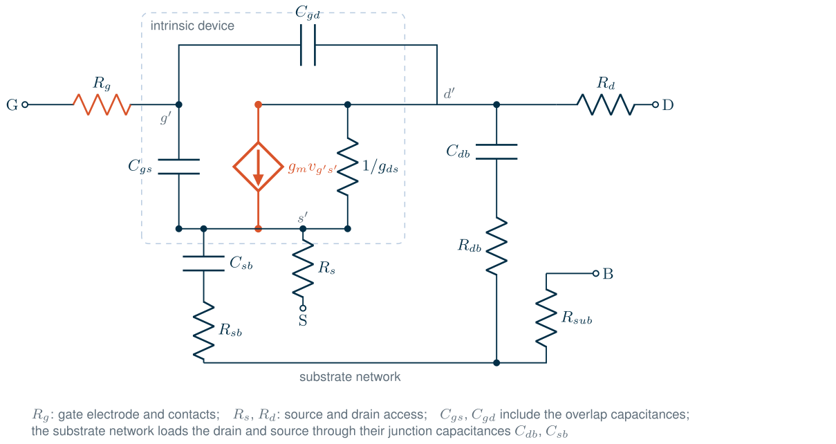
In The Art of Analog IC Design the small-signal MOSFET is a transconductance \(g_m\), an output conductance \(g_{ds}\) and a few capacitances. That model holds up to a few hundred megahertz. At radio frequencies three more things matter (Figure 6.1) [89, 7, 6]:
- The gate resistance \(R_g\). The gate electrode is a thin strip of silicided polysilicon with a sheet resistance of a few ohms per square, fed through contacts. In series with \(C_{gs}\), it absorbs input power and adds thermal noise.
- The substrate network. The drain and source junction capacitances \(C_{db}\) and \(C_{sb}\) do not connect to an ideal ground but to the resistive substrate. Above a few gigahertz they load the drain with a resistance.
- Non-quasi-static (NQS) effects. The channel charge cannot follow the gate voltage instantly. The channel behaves like a distributed RC line, which adds a resistance of the order of \(1/(5g_m)\) in series with \(C_{gs}\) and delays \(g_m\) [89].
The transit frequency
Drive the gate with a current \(i_{in}\) and short the drain to AC ground. The current divides between \(C_{gs}\) and \(C_{gd}\), so \(v_{gs} = i_{in}/j\omega(C_{gs} + C_{gd})\), and the drain delivers \(g_m v_{gs}\). The ratio of the two currents is the short-circuit current gain \(h_{21}\), which falls at 20 dB per decade; the frequency where its magnitude reaches one is the transit frequency:
Key equation · Transit frequency of a MOSFET
\[f_T \approx \frac{g_m}{2\pi\,(C_{gs} + C_{gd})} = \frac{g_m}{2\pi\,C_{gg}}. \tag{6.1}\]\(C_{gg}\) is the total gate capacitance, overlaps included. \(R_g\) does not appear: an ideal current source drives the gate whatever its series resistance.
\(f_T\) is the speed of the transistor itself, the inverse of the time it takes the gate charge to be replaced by the drain current. A useful amplifier at frequency \(f\) needs \(f_T\) well above \(f\); the gain of a common-source stage with a capacitive load falls roughly as \(f_T/f\).
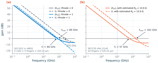
In a simulation, \(\vert h_{21}\vert\) does not keep falling at 20 dB per decade up to its crossing. Above \(f_T\) the current fed straight through \(C_{gd}\) to the shorted drain, which the intrinsic \(g_m\) no longer dwarfs, makes \(\vert h_{21}\vert\) level off at a few tenths. The direct crossing therefore overestimates \(f_T\). The usual practice, and the one in IHP’s process specification [200], is to read \(\vert h_{21}\vert\) and \(U\) at a spot frequency \(f_0\) where both still fall at 20 dB per decade and to extrapolate:
\[f_T = f_0\,\vert h_{21}(f_0)\vert, \qquad f_{max} = f_0\,\sqrt{U(f_0)}. \tag{6.2}\]This chapter uses \(f_0\) = 10 GHz for the MOSFETs and 40 GHz, as IHP does, for the HBTs.
Mason’s unilateral gain and fmax
\(f_T\) says nothing about power. Mason’s unilateral power gain \(U\) is the gain of the transistor after lossless feedback has cancelled its reverse transmission and both ports are matched (Chapter 3) [47]:
\[U = \frac{\vert y_{21} - y_{12}\vert^2}{4\left[\mathrm{Re}(y_{11})\,\mathrm{Re}(y_{22}) - \mathrm{Re}(y_{12})\,\mathrm{Re}(y_{21})\right]}. \tag{6.3}\]No lossless, reciprocal network around the device changes \(U\), so the frequency at which it reaches one, the maximum oscillation frequency \(f_{max}\), is a property of the device: above it no passive embedding can make it amplify power, or oscillate. The denominator of Eq. (6.3) holds the losses: without \(\mathrm{Re}(y_{11})\), that is without \(R_g\), \(U\) is unbounded. For the model of Figure 6.1 (with \(R_s\) = 0) [6, 10]:
Key equation · Maximum oscillation frequency of a MOSFET
\[f_{max} \approx \frac{f_T}{2\sqrt{g_{ds}R_g + 2\pi f_T R_g C_{gd}}} \approx \sqrt{\frac{f_T}{8\pi R_g C_{gd}}}. \tag{6.4}\]The second form neglects \(g_{ds}\). A fast device (\(f_T\)) is not enough: \(f_{max}\) also needs a small gate resistance and a small \(C_{gd}\).
Derivation · fmax of the MOSFET
Make the device unilateral and match it. At the input, \(R_g\) in series with \(C_{gg}\) absorbs the power; with \(v_{gs} = i_{in}/j\omega C_{gg}\), the input power is \(\tfrac12\vert i_{in}\vert^2R_g\). At the output, the drain sees \(g_{ds}\) plus the conductance that \(C_{gd}\) feeds back from the gate: a drain voltage \(v_d\) drives \(j\omega C_{gd}v_d\) into the gate node, which (for \(\omega R_gC_{gg} \ll 1\)) raises \(v_{gs}\) by \(C_{gd}v_d/C_{gg}\) and the drain current by \(g_mC_{gd}v_d/C_{gg} = 2\pi f_TC_{gd}v_d\). The output conductance is \(g_{out} = g_{ds} + 2\pi f_TC_{gd}\), and the matched output power is \(\vert g_mv_{gs}\vert^2/(8g_{out})\). The ratio is
\[U \approx \frac{(f_T/f)^2}{4R_g\,(g_{ds} + 2\pi f_T C_{gd})},\]which falls at 20 dB per decade and reaches one at the \(f_{max}\) of Eq. (6.4). A source resistance \(R_s\) adds to \(R_g\) in the first term; the full expression is in [6].
The S-parameter testbench
Both figures of merit come from the two-port parameters of the device. ngspice’s sp analysis (Chapter 2) computes them between ports, which are voltage sources with a port number and a reference impedance; with a final flag of 1 it also computes the noise parameters (Section 6.5) [194]. Ideal 1 F capacitors and 1 H inductors separate the DC bias from the RF ports. Every MOSFET in this chapter is 20 µm wide, drawn as ten fingers of 2 µm at minimum length; Section 6.2 explains why the SG13G2 device is split into two cells of five fingers.
* ports, DC blocks (1 F) and bias inductors (1 H) around the device
v1  p1 0 dc 0 ac 1 portnum 1 z0 50
v2  p2 0 dc 0 ac 1 portnum 2 z0 50
C1  p1 x1 1
C2  p2 x2 1
Vbi bi 0 0.95                 ; VGS
L1  bi x1 1
Vbo bo 0 0.6                  ; VDS = VDD/2
L2  bo x2 1
XM1 x2 x1 0 0 sg13_lv_nmos W=10u L=0.13u ng=5 m=2 rfmode=1
* HBT instead (.lib cornerHBT.lib hbt_typ):  XQ1 x2 x1 0 0 npn13G2 Nx=4
.control
op
sp dec 20 1e8 1e11 1          ; 0.1-100 GHz; the final 1 adds the noise analysis
.endc
* same ports and bias network; VGS = 1.15 V, VDS = 0.9 V (VDD/2)
* the model has no gate resistance: add the layout estimate of Eq. (6.5)
Rgx x1 xg 12.96
XM1 x2 xg 0 0 sky130_fd_pr__nfet_01v8 W=20 L=0.15 nf=10 ad=... as=... pd=... ps=...
.control
op
sp dec 20 1e8 1e11 1
.endc
Figure 6.2 shows \(\vert h_{21}\vert\) and \(U\) of both MOSFETs at 0.153 mA/µm (SG13G2) and 0.165 mA/µm (SKY130). With its RF model on (rfmode=1, Section 6.2), the SG13G2 device reaches fT = 65.6 GHz and fmax = 89.0 GHz at \(V_{GS}\) = 0.9 V (\(I_D\) = 3.07 mA). With the plain model (rfmode=0), \(f_T\) hardly changes (70.1 GHz) but \(f_{max}\) jumps to 216 GHz, because that model’s only gate resistance is 5.01 Ω. The SKY130 device (\(V_{GS}\) = 1.2 V, \(I_D\) = 3.30 mA) reaches 56.5 GHz. Its model has no gate resistance at all: \(U\) comes out negative below 100 GHz, which only says that Eq. (6.3) has nothing to divide by. With the 13.0 Ω that Section 6.2 estimates from the layout, \(f_{max}\) = 162 GHz. The direct crossings differ from the extrapolations as expected: \(\vert h_{21}\vert\) of the SG13G2 device crosses 0 dB at 73.9 GHz, above the extrapolated 65.6 GHz, and then levels off.
Worked example 6.1 · fT and fmax by hand
Read the model elements of the SG13G2 device at its peak-\(f_{max}\) bias (\(V_{GS}\) = 0.95 V, \(I_D\) = 3.74 mA) from the Y-parameters at 1 GHz (Chapter 3): \(g_m = \mathrm{Re}(y_{21})\) = 13.8 mS, \(g_{ds} = \mathrm{Re}(y_{22})\) = 1.19 mS, \(C_{gg} = \mathrm{Im}(y_{11})/\omega\) = 31.8 fF and \(C_{gd} = -\mathrm{Im}(y_{12})/\omega\) = 11.0 fF (so \(C_{gs}\) = 20.8 fF). The model’s gate resistance is \(R_g\) = 25.5 Ω (Worked example 6.2).
Eq. (6.1): \(f_T\) = 13.8 mS / (2π × 31.8 fF) = 69.2 GHz; the extrapolated simulation gives 69.5 GHz.
Eq. (6.4) without \(g_{ds}\): \(f_{max} = \sqrt{69.2\ \mathrm{GHz}/(8\pi \times 25.5\ \Omega \times 11.0\ \mathrm{fF})}\) = 99.2 GHz. With the \(g_{ds}R_g\) term kept: 88.8 GHz, against 89.7 GHz simulated.
The same steps for the SKY130 device at its peak-\(f_{max}\) bias (\(V_{GS}\) = 1.15 V: \(g_m\) = 9.17 mS, \(g_{ds}\) = 0.77 mS, \(C_{gg}\) = 26.4 fF, \(C_{gd}\) = 4.93 fF, \(R_g\) = 13.0 Ω) give \(f_T\) = 55.2 GHz (55.4 GHz simulated) and \(f_{max}\) = 154 GHz (162 GHz simulated).
Once \(g_{ds}\) is kept, the hand formulas agree with the simulation to a few per cent. SKY130’s higher \(f_{max}\) comes from its smaller \(C_{gd}\) and its smaller (estimated) \(R_g\), not from a faster channel.
6.2 Layout: fingers, gate resistance and SG13G2’s RF model
The gate resistance of a finger
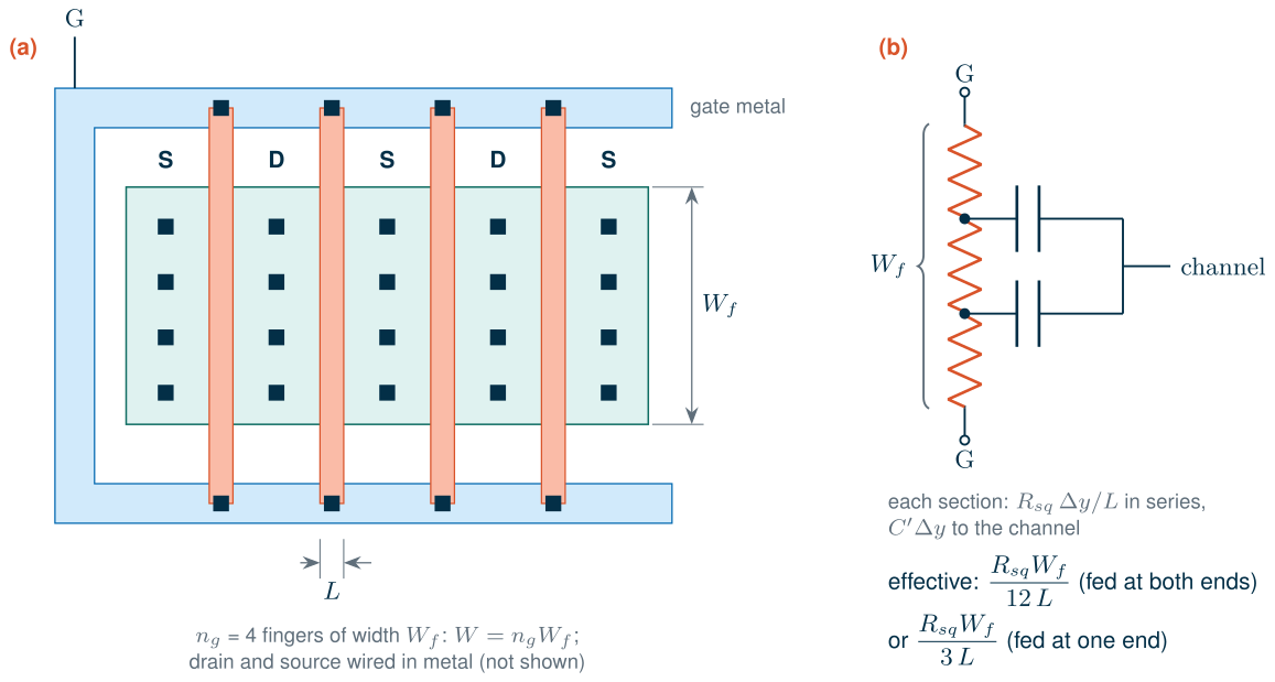
A wide transistor drawn as one long gate would have a hopeless gate resistance. RF transistors are therefore drawn as \(n_g\) parallel fingers of width \(W_f\) that share source and drain diffusions, with the gates joined in metal (Figure 6.3a). Along one finger, the gate is a distributed RC line (Figure 6.3b): every section of length \(\Delta y\) has a series resistance \(R_{sq}\Delta y/L\) and a capacitance to the channel. Because the current that charges the far end flows through all the resistance, but the current to the near end through almost none, the line behaves like a lumped resistance of one third of its total when fed from one end, and one twelfth when fed from both [87]:
\[R_g = \frac{1}{n_g}\left(\frac{R_{sq}W_f}{12\,L} + \frac{R_{con}}{2}\right) \quad \text{(both ends)}, \qquad \frac{1}{n_g}\left(\frac{R_{sq}W_f}{3\,L} + R_{con}\right) \quad \text{(one end)}, \tag{6.5}\]with \(R_{con}\) the resistance of the contact at each end. For a fixed total width \(W = n_gW_f\), the poly term falls as \(1/n_g^2\): halving the finger width halves each finger’s resistance and doubles the number in parallel.
What rfmode=1 adds in SG13G2
IHP ships two model cards for each MOSFET [205]. rfmode=0 selects the PSP 103 model [91] used for analog work; rfmode=1 selects an RF card that differs in four ways:
- Non-quasi-static channel charge, with five collocation points (
swnqs = 5). - Gate resistance: a gate sheet resistance \(R_{SHG}\) = 3 Ω/sq with both ends of each finger contacted, a fixed \(R_{GO}\) = 40 Ω, and the silicide-to-poly interface resistance \(R_{INT}\) = 13.0 Ω µm², the only term present with
rfmode=0. - A substrate network: bulk, well and junction resistances (
rbulko,rwello,rjunso,rjundo) between the internal bulk nodes and the bulk terminal. - Extra gate capacitance: the capacitive width of every finger grows by 0.48 µm, which accounts for the gate’s end caps over the field oxide, and cells of fewer than three fingers get 40 nm of extra capacitive length.
PSP’s scaling equations combine the gate-resistance terms into
\[R_g = \frac{1}{n_g m}\left[\frac{R_{SHG}\,(W_f/6 + X_{GW})}{2L} + \frac{R_{INT}}{W_fL}\right] + \frac{R_{GO}}{m}, \tag{6.6}\]with \(m\) the number of identical cells and \(X_{GW}\) = 0.1 µm the distance from the gate contact to the channel. \(R_{GO}\) is divided by the number of cells, not by the number of fingers.
The substrate network shows in the output conductance: for the device of Figure 6.2, \(\mathrm{Re}(y_{22})\) is 0.979 mS at 1 GHz and 2.45 mS at 50 GHz with rfmode=1, but stays at 1.05 mS with rfmode=0.
Worked example 6.2 · The gate resistance of the reference device
SG13G2, two cells (\(m\) = 2) of five fingers (\(n_g\) = 5), \(W_f\) = 2 µm, L = 0.13 µm, Eq. (6.6). Per finger, the sheet resistance gives 3 Ω/sq × (0.333 + 0.1) µm / 0.26 µm = 5.0 Ω and the interface 13.0 Ω µm² / 0.26 µm² = 50.1 Ω; ten fingers in parallel make 5.5 Ω. The cells add \(R_{GO}/m\) = 20 Ω: Rg = 25.5 Ω, of which the fingers contribute 5.5 Ω and the cells 20 Ω. The simulated input resistance \(\mathrm{Re}(1/y_{11})\) at 10 GHz is 26.5 Ω; the extra ohm is the NQS channel resistance.
SKY130, ten fingers of 2/0.15 µm in one cell, Eq. (6.5) with both ends contacted. The SKY130 model has no gate resistance (
rgatemod = 0), so we estimate it from the poly sheet resistance and the poly-contact resistance of the Magic technology file [201], 48.2 Ω/sq and 152 Ω: 48.2 × 2 / (12 × 0.15) = 53.6 Ω of poly and 152/2 = 76 Ω of contact per finger, Rg = 13.0 Ω for ten fingers. The estimate omits the metal that feeds the fingers.
Fingers against cells
Figure 6.4 puts Eq. (6.6) to work on twelve ways of drawing 20 µm at the bias of peak \(f_{max}\) (\(V_{GS}\) = 0.95 V, 0.187 mA/µm). Drawn as one cell of ten 2 µm fingers, the device has 46.6 Ω of input resistance, nearly all of it \(R_{GO}\); as two cells, 26.5 Ω; as five, 15.5 Ω; as ten single-finger cells, 11.4 Ω. Eq. (6.6) gives 45.5, 25.5, 13.5 and 9.51 Ω; the rest is the NQS channel resistance. With rfmode=0 every layout shows the same 5.01 Ω, \(R_{INT}/WL\), which is why that model’s \(f_{max}\) means nothing.
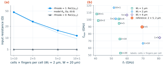
\(f_{max}\) follows the gate resistance: 66.5 GHz for one cell of ten fingers, 89.7 GHz for two cells, 117 GHz for ten single-finger cells. \(f_T\) moves the other way, because of the extra capacitance of the RF card: ten single-finger cells have 42.8 fF of gate capacitance instead of 31.6 fF, and \(f_T\) drops from 70.0 to 51.6 GHz. Wide fingers give the highest \(f_T\): one cell of five 4 µm fingers reaches 80.6 GHz, with 28.7 fF, but only 74.6 GHz of \(f_{max}\). The reference device of this chapter, two cells of five 2 µm fingers, sits at the knee: 69.5 GHz and 89.7 GHz. The noise follows \(R_g\) too (Section 6.5): \(NF_{min}\) at 50 GHz is 4.77 dB for one cell, 3.60 dB for two and 2.98 dB for ten.
Common pitfall · One big instance with many fingers
Writing a 200 µm LNA transistor as one SG13G2 instance with
ng=100gives it the full 40 Ω of \(R_{GO}\), comparable to the 50 Ω source it should match, and a noise figure to match. Split wide RF devices into several cells (themparameter or separate instances), keep at least three fingers per cell, and always simulate RF circuits withrfmode=1. In silicon, what counts is how the fingers are wired; check the final layout with extraction and electromagnetic simulation (Chapter 18).
SG13G2 vs SKY130 · Gate resistance in the models
IHP’s RF card models the gate resistance, the substrate network and NQS effects, fitted to IHP’s RF test structures, so its absolute numbers apply best to layouts like those. SKY130’s
nfet_01v8(BSIM4) has a substrate network (rbodymod = 1) but no gate resistance (rgatemod = 0) and no NQS model, so its \(f_{max}\) and noise come out optimistic unless you add \(R_g\) yourself, as this chapter does with Eq. (6.5). The SKY130 numbers below therefore compare the channels of the two processes more than their finished devices.
6.3 fT and fmax across bias, SG13G2 and SKY130
Speed depends on bias, and the natural bias variable for RF work is the current density \(I_D/W\): at a given \(V_{DS}\), \(f_T\), \(f_{max}\), \(g_m/I_D\) and \(NF_{min}\) all depend on it and not on \(W\) (the \(g_m/I_D\) chapter of the analog course makes the same argument for \(g_m/I_D\)). Figure 6.5 sweeps \(V_{GS}\) of both reference devices at \(V_{DS} = V_{DD}/2\), a typical drain voltage of a cascoded RF stage.
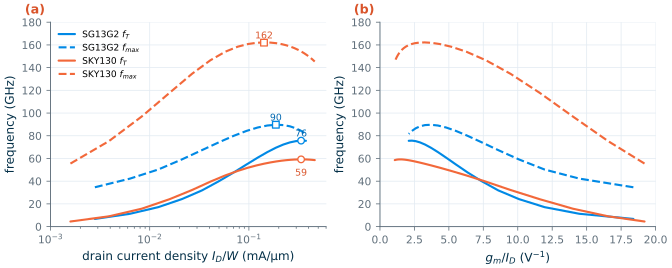
The SG13G2 device peaks at fT = 75.7 GHz at 0.336 mA/µm and fmax = 89.7 GHz at 0.187 mA/µm. At \(V_{DS}\) = 1.2 V they rise to 89.5 GHz (at 0.424 mA/µm) and 109 GHz (at 0.335 mA/µm). The SKY130 device peaks at 59.2 GHz at 0.336 mA/µm and 162 GHz at 0.142 mA/µm, and at \(V_{DS}\) = 1.8 V at 62.9 and 174 GHz. Three things stand out:
- \(f_T\) saturates, \(f_{max}\) turns over. At high current density, velocity saturation stops \(g_m\) from growing while \(C_{gg}\) keeps rising slowly; \(f_{max}\) falls earlier because \(g_{ds}\) rises and the extra current buys no extra \(f_T\) to pay for it in Eq. (6.4).
- The current densities are nearly the same in both processes, and close to the values that Dickson et al. found to hold across CMOS generations: about 0.3 mA/µm for peak \(f_T\), 0.2 mA/µm for peak \(f_{max}\) and 0.15 mA/µm for minimum noise [29, 10]. A design biased by current density keeps its speed when it is resized.
- Peak speed costs efficiency. At peak \(f_T\), \(g_m/I_D\) is only 2.32 V⁻¹ in SG13G2 and 1.48 V⁻¹ in SKY130. Moving to \(g_m/I_D\) = 10 V⁻¹ (0.0218 mA/µm in SG13G2) cuts \(f_T\) to 24.6 GHz in SG13G2 and 30.2 GHz in SKY130, still far above the course radio’s 2.4 GHz.
SG13G2 vs SKY130 · Transit frequency and capacitances
SG13G2’s thinner gate oxide and shorter channel give it more \(g_m\) per micrometre, but also more capacitance: at peak \(f_T\), \(C_{gg}\) is 1.65 fF/µm against 1.34 fF/µm, and \(C_{gd}\) 0.575 fF/µm against 0.248 fF/µm, a \(C_{gd}/C_{gg}\) of 0.349 against 0.184. The large gate–drain capacitance, partly the RF card’s extra end-cap capacitance, limits SG13G2’s peak \(f_T\) to 75.7 GHz against SKY130’s 59.2 GHz, and below about 0.07 mA/µm SKY130 is the faster of the two (Figure 6.5a). For the LNA it also means more Miller feedback, one more reason for the cascode of Chapter 9.
6.4 The SiGe heterojunction bipolar transistor
How it works
Figure 6.6a sketches a modern SiGe HBT. Electrons injected from the n+ polysilicon emitter cross a thin p+ base, a few tens of nanometres of silicon-germanium, then the depleted n− collector, and leave through the buried layer and the sinker. Deep trenches around the device cut its capacitance to the substrate. Germanium does two things [25, 10]:
- It lowers the band gap of the base, so electrons are injected more easily than holes flow back: the current gain \(\beta\) is high even with a heavily doped base, and a heavily doped base has a low base resistance \(r_b\).
- Its content is graded across the base, which builds in an electric field that accelerates the electrons: the base transit time shrinks severalfold compared with a silicon transistor of the same base width.
IHP has described HBTs of this class, with fT/fmax of 300/500 GHz, in [92]. The process specification gives the high-speed npn13G2 (emitter 0.07 × 0.9 µm² per finger) fT = 350 GHz and fmax = 450 GHz (typical, four fingers, \(V_{CE}\) = 1.2 V, extrapolated from 40 GHz), the npn13G2l with longer emitters 330/430 GHz, and the higher-voltage npn13G2v 120/330 GHz [200]. IHP models all three with VBIC [41, 205], including self-heating, quasi-saturation and weak avalanche.
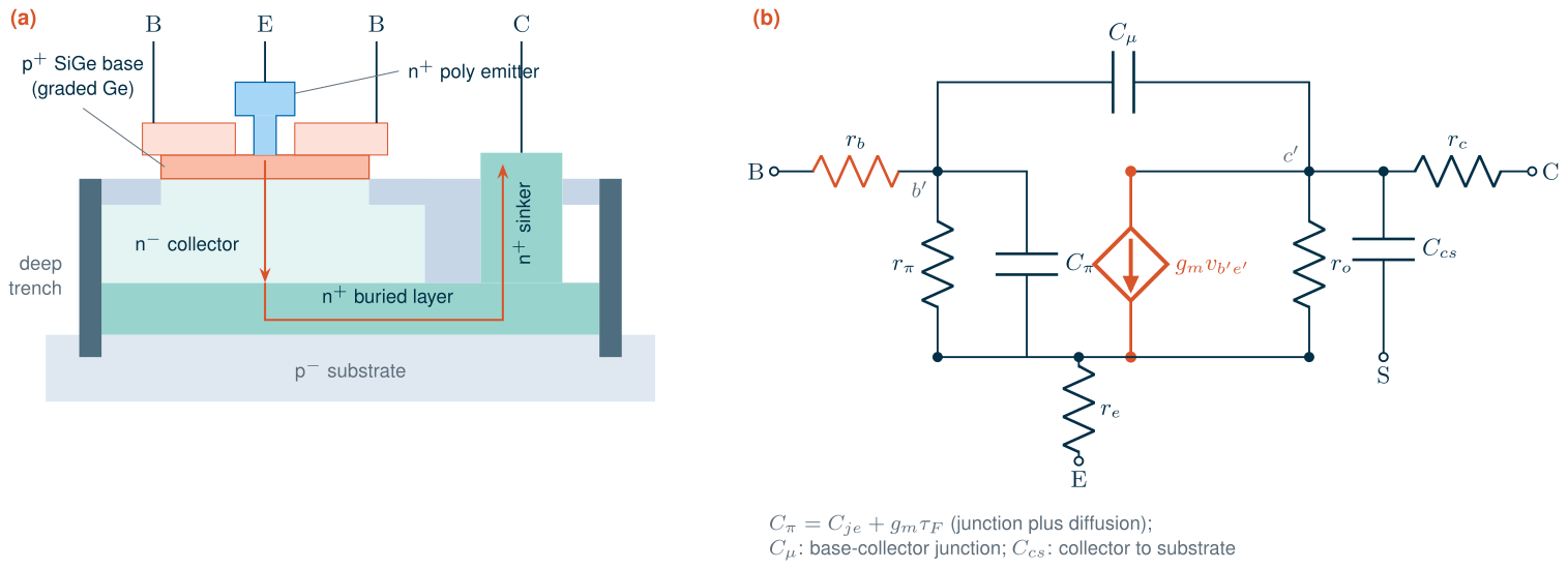
The hybrid-π model of Figure 6.6b gives the bipolar version of Eq. (6.1). With \(C_\pi = C_{je} + g_m\tau_F\) and \(g_m = I_C/V_T\), the time to charge the input splits into a part fixed by the device and parts that shrink with current [10]:
Key equation · Transit time of a bipolar transistor
\[\frac{1}{2\pi f_T} = \tau_F + \frac{V_T}{I_C}\,(C_{je} + C_\mu) + C_\mu\,(r_e + r_c). \tag{6.7}\]At low current the junction capacitances dominate and \(f_T\) rises in proportion to \(I_C\); at high current it approaches \(1/2\pi[\tau_F + C_\mu(r_e + r_c)]\).
The argument behind Eq. (6.4) carries over to \(f_{max}\), with the base resistance in place of \(R_g\) and \(C_\mu\) in place of \(C_{gd}\) (\(g_o\) negligible):
\[f_{max} \approx \sqrt{\frac{f_T}{8\pi\,r_b\,C_\mu}}. \tag{6.9}\]fT and fmax against current density
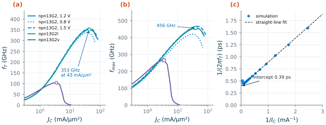
Figure 6.7 shows the three HBTs, four emitter fingers each, against the collector current density \(J_C = I_C/A_E\) on the drawn emitter area (0.252 µm² for npn13G2). At \(V_{CE}\) = 1.2 V the npn13G2 peaks at fT = 353 GHz at 42.8 mA/µm² (\(I_C\) = 10.8 mA, \(\beta\) = 363) and fmax = 456 GHz at 38.1 mA/µm², on top of IHP’s typical values. The npn13G2l (le = 1 µm) is almost identical, 352 and 457 GHz. The npn13G2v (le = 1 µm) reaches 104 and 265 GHz at only 3.51 mA/µm²: its \(f_T\) lies between IHP’s minimum and typical values (90 and 120 GHz), its \(f_{max}\) somewhat below the specified minimum of 280 GHz.
Worked example 6.3 · Reading the transit time from simulation
Eq. (6.7) is a straight line in \(1/I_C\). The fit of Figure 6.7c has a slope of \(V_T(C_{je} + C_\mu)\) with \(C_{je} + C_\mu\) = 19.2 fF, and an intercept of 0.393 ps, so even with infinite current \(f_T\) could not exceed 1/(2π × 0.393 ps) = 405 GHz. The model card gives \(\tau_F\) = 0.208 ps; with \(C_\mu\) = 7.38 fF (from \(y_{12}\)) and \(r_e + r_c\) = 33.0 Ω (the card’s \(r_e\), \(r_{cx}\) and \(r_{ci}\) for four emitters), \(C_\mu(r_e + r_c)\) = 0.244 ps and Eq. (6.7) predicts 0.452 ps, against 0.393 ps from the fit. The collector charging the base–collector capacitance takes longer than the electrons take to cross the base: in a fast HBT the parasitics matter as much as the base.
\(f_{max}\) by hand, Eq. (6.9), with the card’s \(r_b = r_{bx} + r_{bi}\) = 28.9 Ω and \(C_\mu\) = 7.35 fF gives 257 GHz, against 456 GHz simulated. The simple formula is pessimistic: the intrinsic base resistance falls at high current, and part of \(C_\mu\) connects to the external base, behind only \(r_{bx}\). For HBTs, trust the simulation.
The Kirk effect
Why does \(f_T\) fall above its peak? The electrons crossing the collector depletion region carry a charge density \(J_C/v_{sat}\). When it approaches the collector doping \(qN_C\), the field at the base–collector junction collapses and the neutral base pushes out into the collector. The base becomes wider, \(\tau_F\) grows, and \(f_T\) falls: the Kirk effect [85]. The current density where it starts grows with the collector doping and with the reverse voltage across the collector [10]:
\[J_K \approx q\,N_C\,v_{sat}\left[1 + \frac{2\varepsilon_{Si}\,(V_{CB} + \phi_{bi})}{q\,N_C\,W_C^2}\right]. \tag{6.8}\]Figure 6.7a shows both dependences. Raising \(V_{CE}\) from 0.8 to 1.5 V moves the point where \(f_T\) has fallen to 90 % of its peak from 66.3 to 77.5 mA/µm². The npn13G2v has a lighter, wider collector so that it can hold more voltage; by Eq. (6.8) its Kirk current density is far lower, and its \(f_T\) collapses above 5.56 mA/µm². In VBIC the roll-off comes from high-level injection (ikf) and the quasi-saturation model of the collector (rci, vo, gamm) [41]. The practical rule: bias an HBT on the rising side of its \(f_T\) curve, below the peak, where the device is fast and well behaved.
Breakdown and the power-amplifier supply
The thin, heavily doped layers that make the HBT fast also make it fragile. IHP specifies, typical (minimum) [200]:
npn13G2andnpn13G2l: \(BV_{CEO}\) = 1.6 V (1.4 V), \(BV_{CBO}\) = 4.8 V (3.8 V);npn13G2v: \(BV_{CEO}\) = 2.5 V (2.2 V), \(BV_{CBO}\) = 8.5 V (7 V).
\(BV_{CBO}\) is the avalanche breakdown of the base–collector junction. With the base open, it comes much earlier: the holes that the avalanche generates in the collector flow into the base, and with nowhere else to go they act as base current, which the transistor multiplies by \(\beta\). Breakdown occurs when the multiplication factor \(M\) satisfies \(\beta(M - 1) = 1\); with the empirical \(M = 1/[1 - (V_{CB}/BV_{CBO})^n]\) [90, 10],
\[BV_{CEO} \approx \frac{BV_{CBO}}{\beta^{1/n}}, \qquad n \approx 3\text{–}6. \tag{6.10}\]VBIC models the weak avalanche as a current proportional to \(I_C\), so the models reproduce \(BV_{CEO}\) but not \(BV_{CBO}\) (with the emitter open there is no current to multiply). Figure 6.8 shows both views of the same effect, with self-heating switched off. With the base current forced, the collector current of npn13G2 runs away above 1.6 V and doubles from its 1 V value at 1.88 V. With \(V_{BE}\) forced, the avalanche holes flow out of the base terminal, and the base current reverses at 1.62 V (npn13G2), 1.63 V (npn13G2l) and 2.60 V (npn13G2v), on top of the specified \(BV_{CEO}\).
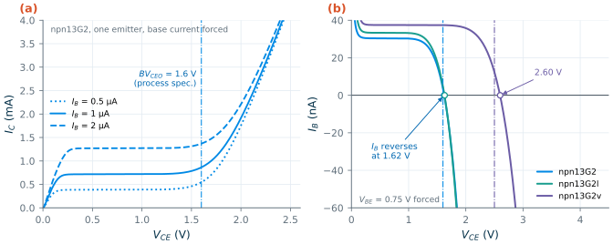
The reversal voltage depends a little on the bias (1.58 to 1.68 V for npn13G2 between \(V_{BE}\) = 0.70 and 0.80 V) and much more on the base drive. A base fed from a low impedance can sink the avalanche current, so the usable collector voltage rises from \(BV_{CEO}\) towards \(BV_{CBO}\), until other instabilities set in [90]. This is what limits a power amplifier. In a class-A or class-B stage the collector swings from near zero to about twice the supply, so, neglecting the knee voltage, \(V_{CC} \le BV/2\) and the load for an output power \(P\) is \(R_L = V_{CC}^2/2P\). For the course transmitter’s +10 dBm, Table 6.1 gives the supply and load.
Table 6.1. Supply and load of a class-A or class-B HBT stage for +10 dBm, if the collector may swing to BVCEO or to BVCBO (typical values of the process specification; knee voltage neglected).
| Limit | npn13G2 | npn13G2v |
|---|---|---|
| Peak at BVCEO: VCC, RL | 0.8 V, 32.0 Ω | 1.25 V, 78.1 Ω |
| Peak at BVCBO (low-impedance base): VCC, RL | 2.4 V, 288 Ω | 4.25 V, 903 Ω |
A stage whose collector stays below \(BV_{CEO}\) needs a load below 50 Ω, which means a lossy impedance transformation; designs that drive the base from a low impedance can use a higher supply and a load near 50 Ω, at the price of a careful reliability analysis. Chapter 16 makes this choice for the course PA, and Chapter 17 for the 50 GHz amplifier. The 1.2 V MOSFETs are no easier: their drain breakdown \(BV_{DSS}\) is 2.7 V typical and 2.0 V minimum, and the 3.3 V devices reach 6.1 V (5.3 V) but only 16.0 GHz of \(f_T\) [200].
6.5 Noise parameters
Four numbers for a noisy two-port
Any linear noisy two-port can be described by its noiseless self plus two correlated noise sources at its input. Its noise factor then depends on the source admittance \(Y_s = G_s + jB_s\) through four noise parameters: the minimum noise factor \(F_{min}\), the optimum source admittance \(Y_{opt}\) (two numbers) at which it occurs, and the noise resistance \(R_n\) that sets how fast \(F\) rises away from it [63, 9]. In terms of reflection coefficients relative to \(Z_0\):
Key equation · Noise factor of a two-port
\[F = F_{min} + \frac{R_n}{G_s}\,\vert Y_s - Y_{opt}\vert^2 = F_{min} + \frac{4R_n}{Z_0}\,\frac{\vert\Gamma_s - \Gamma_{opt}\vert^2}{(1 - \vert\Gamma_s\vert^2)\,\vert 1 + \Gamma_{opt}\vert^2}. \tag{6.11}\]\(NF_{min} = 10\log_{10}F_{min}\). A small \(R_n\) makes the noise figure forgiving of a mismatched source.
The sp analysis with the noise flag returns, for every frequency, nf (the noise figure with a 50 Ω source), nfmin, rn and sopt [194]. Before trusting units, check them: rebuilding nf from nfmin in dB, rn in ohms and sopt as \(\Gamma_{opt}\) relative to the 50 Ω of port 1, with Eq. (6.11) and \(\Gamma_s\) = 0, reproduces ngspice’s nf to within \(3\times10^{-15}\) dB. So nfmin and nf are in dB, rn is in ohms (not normalized), and sopt is a reflection coefficient. Chapter 4 defines noise figure itself.
The noise sources are different in the two devices. In a MOSFET they are the thermal noise of the channel, the noise it induces on the gate through \(C_{gs}\), and the thermal noise of \(R_g\) and \(R_s\). Fukui’s empirical form captures how they scale [86, 10]:
\[F_{min} \approx 1 + K\,\frac{f}{f_T}\sqrt{g_m\,(R_g + R_s)}, \tag{6.12}\]with a fitting factor \(K\) of order 2. In a bipolar transistor they are the shot noise of the base and collector currents and the thermal noise of \(r_b\) and \(r_e\), which give [88]
\[F_{min} \approx 1 + \frac{1}{\beta} + \sqrt{2 g_m (r_b + r_e)\left(\frac{f^2}{f_T^2} + \frac{1}{\beta}\right) + \frac{1}{\beta}}. \tag{6.13}\]Both say the same thing: noise rises with \(f/f_T\) and with the series resistance at the input, so the quiet device is the fast one with a small gate or base resistance.
What the simulations show
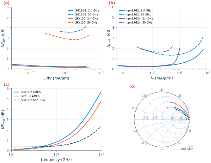
Figure 6.9 collects the results. At 2.4 GHz every device is nearly noiseless: the minimum over bias is 0.200 dB for the SG13G2 nMOS (at 0.153 mA/µm), 0.146 dB for SKY130 (0.189 mA/µm) and 0.224 dB for the npn13G2 (0.552 mA/µm², where its \(f_T\) is only 41.4 GHz). At 50 GHz they separate: 3.55 dB for the SG13G2 nMOS (0.123 mA/µm), 2.83 dB for SKY130 (0.165 mA/µm) and 1.33 dB for the npn13G2 (4.28 mA/µm²). The noise-optimum current densities lie below those of peak \(f_{max}\), in line with the characteristic current densities of Section 6.3.
Eq. (6.12) predicts \(F_{min} - 1 \propto f\) at fixed bias. For the SG13G2 device at 0.123 mA/µm, \(F_{min} - 1\) grows 26.7 times from 2.4 to 50 GHz, a frequency ratio of 20.8: roughly linear, a little faster as \(f\) approaches \(f_T\) = 60.7 GHz. For the HBT, Eq. (6.13) with the card’s \(r_b + r_e\) = 36.1 Ω gives 0.237 dB at the 2.4 GHz optimum (\(I_C\) = 0.139 mA, \(\beta\) = 817), against 0.224 dB simulated, and 1.67 dB at the 50 GHz optimum (1.08 mA), against 1.33 dB; as for \(f_{max}\), the falling intrinsic base resistance makes the formula pessimistic at high current.
Where must the source be? At 2.4 GHz \(\Gamma_{opt}\) of the 20 µm SG13G2 device is 0.981 ∠ 2.07°, near the open circuit: \(Z_{opt}\) = 1160 + j2140 Ω. At 50 GHz it moves to 0.670 ∠ 38.7°, \(Z_{opt}\) = 68.3 + j104 Ω. \(R_n\) is 118 Ω and 104 Ω. The HBT’s \(Z_{opt}\) is 1320 + j338 Ω and 131 + j162 Ω, with \(R_n\) = 55.9 and 55.2 Ω.
Worked example 6.4 · Sizing a device for noise matching
At constant current density, \(NF_{min}\) does not depend on the width, while \(R_n\) and \(Z_{opt}\) scale as \(1/W\): \(W\) fingers in parallel are \(W\) identical noisy two-ports in parallel. The simulation confirms it: doubling the SG13G2 device to 40 µm at the same \(V_{GS}\) halves \(R_n\) from 118 to 59.0 Ω and \(Z_{opt}\) from 1160 + j2140 to 582 + j1070 Ω, with \(NF_{min}\) unchanged at 0.201 dB.
To bring \(\mathrm{Re}(Z_{opt})\) to 50 Ω at 2.4 GHz by size alone, the nMOS would need \(W\) = 20 µm × 1160/50 = 464 µm, drawing 57.1 mA at 0.123 mA/µm, and the HBT 106 emitter fingers (28.5 mA). At 50 GHz, 27.3 µm (3.36 mA) or 10.5 fingers (2.83 mA) suffice. At millimetre waves, sizing the device is the noise match; at 2.4 GHz it would waste tens of milliamperes and still leave the large reactance to tune out. That is why the course LNA uses inductive source degeneration instead, which turns the gate’s reactive input into a resistance without changing \(\Gamma_{opt}\) much (Chapter 9).
What this means for your design
At 2.4 GHz noise is not limited by the transistor’s speed: the SG13G2 nMOS has \(NF_{min}\) = 0.270 dB even at \(g_m/I_D\) = 10 V⁻¹, where each milliampere buys 10 mS instead of the 4.2 mS at its noise optimum. The losses of the matching network and the gate wiring will dominate, so bias the LNA for gain and power, not for the last 0.1 dB of \(NF_{min}\). At 50 GHz every tenth of a dB counts, the HBT’s 1.33 dB beats the nMOS’s 3.55 dB, and its noise-optimum current density (4.28 mA/µm²) lies far below that of peak \(f_T\) (42.8 mA/µm²).
6.6 Choosing a device for each block
Table 6.2 collects the simulated metrics, and Table 6.3 turns them into a choice of device for each block of the course radio at 2.4 GHz and of a 50 GHz front end.
Table 6.2. Simulated device metrics (typical models, 27 °C; fT and fmax extrapolated from 10 GHz for MOSFETs and 40 GHz for HBTs). MOSFETs 20 µm wide in 2 µm fingers at VDS = VDD/2 (SG13G2 3.3 V nMOS: L = 0.45 µm, VDS = 1.65 V); HBTs Nx = 4 at VCE = 1.2 V. Current densities in mA/µm (MOSFETs) or mA/µm² of drawn emitter area (HBTs). Breakdown voltages from the process specification.
| SG13G2 lv nMOS | SKY130 nfet_01v8 | SG13G2 hv nMOS | npn13G2 | npn13G2v | |
|---|---|---|---|---|---|
| Peak fT (at J) | 75.7 GHz (0.336) | 59.2 GHz (0.336) | 16.0 GHz (0.241) | 353 GHz (42.8) | 104 GHz (3.51) |
| Peak fT at VDS = VDD | 89.5 GHz (0.424) | 62.9 GHz (0.331) | |||
| Peak fmax (at J) | 89.7 GHz (0.187) | 162 GHz (0.142)* | 71.6 GHz (0.0742) | 456 GHz (38.1) | 265 GHz (3.51) |
| Input series resistance | Rg = 25.5 Ω | Rg = 13.0 Ω* | rb = 28.9 Ω | ||
| Min. NFmin at 2.4 GHz (at J) | 0.200 dB (0.153) | 0.146 dB (0.189)* | 0.224 dB (0.552) | 0.22 dB (0.369) | |
| Min. NFmin at 50 GHz (at J) | 3.55 dB (0.123) | 2.83 dB (0.165)* | 1.33 dB (4.28) | 1.63 dB (1.46) | |
| Supply / breakdown | 1.2 V; BVDSS 2.7 V | 1.8 V | 3.3 V; BVDSS 6.1 V | BVCEO 1.6 V, BVCBO 4.8 V | BVCEO 2.5 V, BVCBO 8.5 V |
* SKY130 with the gate resistance estimated from the layout (Worked example 6.2); its model has neither gate resistance nor NQS effects, so these numbers are optimistic.
Table 6.3. Which SG13G2 device for which block, at 2.4 GHz (the course radio) and at 50 GHz, with the reason from this chapter's numbers.
| Block | 2.4 GHz | 50 GHz |
|---|---|---|
| LNA | lv nMOS cascode: NFmin 0.200 dB, fT 75.7 GHz, runs from 1.2 V (Chapter 9); npn13G2 is as quiet (0.224 dB) | npn13G2: NFmin 1.33 dB against 3.55 dB for the nMOS, and a Zopt near 50 Ω with 10.5 emitter fingers |
| Mixer | lv nMOS switches of a passive mixer: speed to spare, no DC current, low flicker noise at the switch (Chapter 10) | npn13G2 Gilbert cell: an LO switch needs fT many times the LO frequency, which only the HBT has |
| VCO | lv nMOS (and pMOS) cross-coupled pair at 4.8 GHz: plenty of gain at 1.2 V, the least parasitic capacitance per mS for the tank (Chapter 11) | npn13G2: an oscillator needs gain at f, so fmax far above it (456 against 89.7 GHz) |
| Divider | lv nMOS CML or TSPC divide-by-two at 4.8 GHz: fT = 75.7 GHz against a 4.8 GHz input (Chapter 13) | npn13G2 CML (emitter-coupled) latches at 42.8 mA/µm², the peak of fT |
| PA | npn13G2v (BVCEO 2.5 V, fmax 265 GHz), the 3.3 V nMOS (BVDSS 6.1 V, fT 16.0 GHz), or a cascode of lv nMOS; never one lv nMOS swinging past 2.0 V (Chapter 16) | npn13G2 (fmax 456 GHz), cascoded or stacked to share the voltage, VCE kept near BVCEO (Chapter 17) |
The pattern is simple. At 2.4 GHz the 1.2 V MOSFET is fast enough for everything, shares the supply and the digital logic of the synthesizer, and costs no extra mask steps, so the course radio’s receiver and synthesizer are CMOS; only the power amplifier needs a higher-voltage device. At 50 GHz the MOSFET runs out of gain and its noise rises steeply, and the HBT, with 456 GHz of \(f_{max}\) against 89.7 GHz and an \(NF_{min}\) of 1.33 dB against 3.55 dB, takes over every block.
Try it · The transistor script
Every number in this chapter comes from
tools/figs/ch06_rf_transistors.py:python3 tools/figs/ch06_rf_transistors.pyredraws everything from the cached simulations,--resimreruns them. Three experiments: (1) inREF, draw the SG13G2 device as one cell (w=20.0, ng=10, m=1) and rerunmos noise --resim: how much do \(f_{max}\) and \(NF_{min}\) at 50 GHz change, and does \(f_T\)? (2) SetSKY_RCONto 0 and rerunmos: how much of SKY130’s estimated \(f_{max}\) depends on the contacts? (3) Add thenpn13G2at \(V_{CE}\) = 1.0 V toHBTSand rerunhbt: where does the Kirk roll-off start now?
- fT = gm/2πCgg measures the speed of the channel; fmax ≈ √(fT/8πRgCgd) measures power gain and depends just as much on the gate resistance and Cgd. Extract both from the current gain h21 and Mason’s U at a spot frequency, extrapolating at −20 dB/decade.
- Layout sets Rg: narrow fingers contacted at both ends, and, in SG13G2’s RF model, several cells, because each cell carries a fixed 40 Ω. Simulate RF circuits with
rfmode=1; without it SG13G2’s fmax comes out 216 instead of 89.0 GHz.- Bias MOSFETs by current density: peak fT near 0.34 mA/µm, peak fmax near 0.14–0.19 mA/µm and minimum noise near 0.12–0.19 mA/µm in both PDKs. The reference SG13G2 nMOS reaches 75.7 GHz fT and 89.7 GHz fmax at VDS = 0.6 V.
- The SiGe HBT reaches 353 GHz fT and 456 GHz fmax, until the Kirk effect stops it; the price is a BVCEO of 1.6 V (2.5 V for npn13G2v), which halves the supply a power amplifier can use.
- At 2.4 GHz every device has an NFmin near 0.2 dB, and CMOS is the natural choice; at 50 GHz the HBT’s 1.33 dB beats the nMOS’s 3.55 dB, and the HBT takes over every block.
Further reading
- S. Voinigescu, High-Frequency Integrated Circuits [10]: the MOSFET and SiGe HBT as RF devices, characteristic current densities and the design of millimetre-wave circuits with them, the closest companion to this chapter.
- C. Enz and Y. Cheng, “MOS transistor modeling for RF IC design” [89]: the gate resistance, substrate network and NQS effects of Figure 6.1, and how compact models include them; B. Razavi, R.-H. Yan and K. F. Lee [87] for the distributed gate resistance of Eq. (6.5).
- T. O. Dickson et al. [29]: why the current densities of peak fT, peak fmax and minimum noise stay nearly constant across CMOS generations, and how to design with them.
- J. D. Cressler [25] on how SiGe HBTs work, and S. P. Voinigescu et al. [88] on their noise and on sizing them for LNAs; M. Rickelt, H.-M. Rein and E. Rose [90] on how far beyond BVCEO a bipolar transistor can safely be driven.