Chapter 17
Millimetre-Wave Design: a 50 GHz Power Amplifier
At 50 GHz a TopMetal2 line is a tenth of a wavelength long after 310 µm, a pad is a 106 Ω reactance and a MIM capacitor can be self-resonant. This chapter designs a one-stage SiGe medium-power amplifier for 50 GHz in the order of the IHP Analog Academy's module: bias and stability, matching with ideal elements, then with TopMetal2 lines and RF MIM capacitors, large-signal simulation, and what the layout and electromagnetic simulation add.
- Explain what changes between 2.4 GHz and 50 GHz: wavelength, pads, MIM parasitics, and the gain left in the transistor.
- Choose the size and bias of an HBT stage from its fT, fmax, MSG/MAG and stability factor.
- Stabilize a common-emitter stage with a series R‖C network and check μ > 1 from 0.1 to 400 GHz.
- Design stub-and-line matching networks, first with ideal elements and then with lossy TopMetal2 lines and cap_rfcmim, and explain where the loss comes from.
- Simulate P1dB, Psat and PAE at 50 GHz, and judge the design against a stated target.
Contents
- 17.1 What changes at millimetre waves
- 17.2 The SiGe HBT at 50 GHz
- 17.3 Biasing and stability
- 17.4 Matching with ideal elements, then with TopMetal2
- 17.5 Large-signal performance
- 17.6 From ideal elements to layout: what EM adds
- 17.7 Results and lessons
- 17.8 A redesign with EM in the loop
- Further reading
17.1 What changes at millimetre waves
The course radio of Parts III to V works at 2.44 GHz, where everything on the chip except the spirals is a lumped node. At 50 GHz, in the band used for short-range links and sensing, that picture breaks in four places. Table 17.1 puts numbers on them, all from the SG13G2 data of earlier chapters.
Table 17.1. The same SG13G2 objects at 2.44 GHz and at 50 GHz (TopMetal2 line of Chapter 7; pad of Chapter 8; cap_rfcmim in ngspice; the transistor of Section 17.2). The design uses the 30 fF estimate; [Chapter 18](/rfic-design/chapters/18-rf-layout/#gsg-pads-and-their-capacitance) finds 37.7 fF at 50 GHz by EM, −j84.4 Ω.
| Object | At 2.44 GHz | At 50 GHz |
|---|---|---|
| Wavelength on the 16 µm TopMetal2 microstrip | 5.61 cm | 3.1 mm (λ/4 = 776 µm) |
| Line loss | 0.283 dB/mm | 0.583 dB/mm |
| 30 fF pad | −j2170 Ω (invisible) | −j106 Ω (part of the match) |
| 3 pH of emitter lead | 0.077 Ω | 0.942 Ω |
| cap_rfcmim 20 µm × 20 µm (603 fF) | 0.60 − j108 Ω | 0.852 + j0.385 Ω (self-resonant near 48 GHz) |
| cap_rfcmim 10 µm × 10 µm (152 fF) | 0.566 − j430 Ω | 0.757 − j16.7 Ω (an ideal 152 fF: −j21.0 Ω) |
| MSG of the 16-emitter npn13G2 stage | 28.5 dB | 15.4 dB |
Every interconnect is a line. A connection longer than about a tenth of a wavelength, 310 µm here, transforms impedances (Chapter 3), so the wiring between the pad, the capacitors and the transistor is part of the matching network; the networks of this chapter are built from it. Pads and capacitors are no longer what they say. The pad’s 30 fF must be absorbed in the match, and a MIM capacitor’s series inductance cancels a growing part of its reactance: the 20 µm capacitor is a near-perfect short at 50 GHz, ideal for decoupling, and the 10 µm one looks like 190 fF instead of 152 fF. The transistor has little gain to spare. Of the 28.5 dB the stage could deliver at 2.44 GHz, 15.4 dB remain at 50 GHz, before stabilization and matching losses. And a few picohenries matter: 3 pH in the emitter is almost an ohm of reactance in series with an input resistance of about 5 Ω.
The design follows the four parts of the IHP Analog Academy’s module 2, a 50 GHz medium-power amplifier (MPA) in SG13G2 with Qucs-S, ngspice, Xyce and openEMS [3]: biasing and stability, ideal matching, nonlinear analysis, and layout with EM simulation. Our circuit, values and figures are our own; the textbook background is in Voinigescu [10] and, for the PA side, Cripps [13]. The target, in the spirit of the academy module, is given in Table 17.3: at 50 GHz, small-signal gain ≥ 10 dB, S11 and S22 ≤ −10 dB, P1dB ≈ +10 dBm, Psat ≥ +10 dBm, and unconditional stability.
17.2 The SiGe HBT at 50 GHz
The transistor is the high-speed npn13G2. Chapter 6 found its fT peak of 353 GHz at 42.8 mA/µm² (Nx = 4, VCE = 1.2 V) and its breakdown voltages BVCEO = 1.6 V and BVCBO = 4.8 V. For about +10 dBm into a load near 50 Ω the collector must swing about 1 V and carry about 20 mA of fundamental current, so the stage uses four instances of Nx = 4 in parallel (16 emitters, 1.01 µm²). Parallel Nx = 4 instances, not one large device, follow the model’s scaling and avoid the convergence problems Chapter 16 met with large Nx. The supply is VCC = 1.5 V, chosen in Section 17.5 from the load line. At VBE = 0.90 V the stage draws 27.5 mA (27.3 mA/µm², β = 466), on the rising side of the fT curve, below the Kirk knee, so that the current peaks of a large signal still find a fast device.
An ngspice sp of the bare stage from 0.1 to 400 GHz (Figure 17.2a) gives fT = 344 GHz and fmax = 455 GHz (extrapolated from 40 GHz at −20 dB/decade), close to the Chapter 6 peaks. At 50 GHz, \(\vert h_{21}\vert^2\) = 16.8 dB, Mason’s U = 19.2 dB and the MSG of Eq. (3.22) is 15.4 dB, but the Rollett factor is only K = 0.387: the device is potentially unstable at 50 GHz, and it stays so up to 138 GHz. Its input impedance at 50 GHz is 5.47 − j5.42 Ω, small because the device is large.
17.3 Biasing and stability
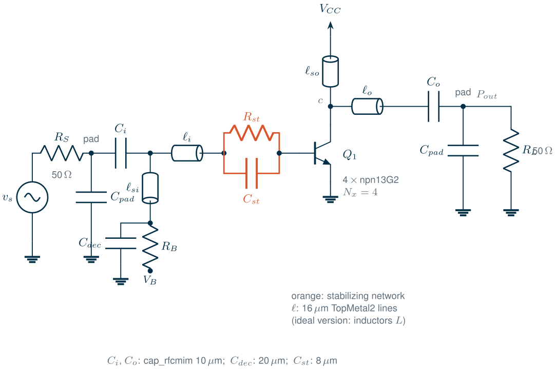
A conditionally stable stage can oscillate when a pad, a probe or the next block presents the wrong impedance, at any frequency where the device has gain, which for this HBT means from DC to beyond 100 GHz. The academy module, like most SiGe millimetre-wave designs, adds loss where the device is unstable and as little as possible where it must amplify [3, 10]. Our network is a resistor \(R_{st}\) in parallel with a capacitor \(C_{st}\) in series with the base:
\[Z_{st} = \frac{R_{st}}{1 + j\omega R_{st}C_{st}}, \qquad f_{st} = \frac{1}{2\pi R_{st}C_{st}}. \tag{17.1}\]Below \(f_{st}\) the resistor is in series with the base and damps the high low-frequency gain; above it the capacitor bypasses most of the resistor, but not all: at 50 GHz, with \(R_{st}\) = 100 Ω and \(C_{st}\) = 100 fF (\(f_{st}\) = 15.9 GHz), \(Z_{st}\) = 9.16 − j28.8 Ω, and the 9.16 Ω are what makes the stage stable at 50 GHz. A search over \(R_{st}\), \(C_{st}\) and an extra series resistor in the script picked these values as the highest-gain choice that keeps μ (Eq. 3.24) above 1 from 20 to 400 GHz with some margin: the stabilized core has μ ≥ 1.06 above 20 GHz (minimum at 77.6 GHz), K = 1.21 at 50 GHz and a MAG of 12.6 dB, 2.8 dB below the bare MSG (Figure 17.2). That is the price of stability, and the gain target leaves only 2.6 dB for the matching networks.
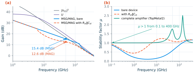
sp, 4 × npn13G2 (Nx = 4), VCE = 1.5 V, IC = 27.5 mA. (a) |h21|², U and MSG/MAG of the bare stage, and MSG/MAG with Rst‖Cst (ideal elements). (b) μ of the bare stage, of the stage with Rst‖Cst, and of the complete TopMetal2 amplifier between its pads.Below a few gigahertz the stabilized core is still potentially unstable (μ = 0.438). The bias network takes care of it. The base is fed through the input stub from a bias node that is decoupled by a 20 µm MIM capacitor and connected to \(V_B\) through \(R_B\) = 100 Ω. At 50 GHz the capacitor shorts the stub’s end; at low frequencies it is open, and the base sees \(R_B\) + \(R_{st}\). The collector is fed through the output stub from the supply, which shorts it at low frequencies. With both networks in place, the complete amplifier has μ ≥ 1 from 0.1 to 400 GHz (Figure 17.2b): it approaches 1 only below a few gigahertz, where the DC blocks disconnect the ports, and above 300 GHz, where the device has no gain left.
Common pitfall · Stabilizing with an ideal capacitor
In the TopMetal2 version, \(C_{st}\) is an 8 µm cap_rfcmim, 97.3 fF at low frequency. Its series inductance makes it look like 111 fF at 50 GHz, which bypasses more of \(R_{st}\): the core alone then has μ = 0.996 at 87.1 GHz, marginally unstable. The complete amplifier is still stable, because its networks add loss there, but the margin a designer counted on with ideal elements has gone. Check stability with the PDK’s RF models, not with the ideal values.
17.4 Matching with ideal elements, then with TopMetal2
Topology
Both networks of Figure 17.1 have the same shape: a shunt element that is also the bias feed, a series element, a DC-blocking capacitor and the pad. On the input, a shorted stub on the 50 Ω side, behind the DC block, and a series line towards the base transform the 50 Ω source down to the low input impedance of the stabilized core, 6.47 − j38.8 Ω. On the output, the stub sits at the collector, where it also resonates the device’s output capacitance, and a series line with the DC block and the pad sets the load resistance. The design solves the four element values for two conditions at 50 GHz:
\[Z_{in}(\text{port 1}) = 50\ \Omega, \qquad Y_L(\text{collector}) = \frac{1}{R_L} - j\,\mathrm{Im}\,Y_{out}, \tag{17.2}\]where \(Y_{out}\) is the output admittance of the core with its input network. The output condition is the load-line match of Chapter 16, Eq. (16.5): the collector sees a resistance \(R_L\) chosen for power, with the output capacitance tuned out, not a conjugate match. With lossy elements the input condition must be imposed at the port: a conjugate match at the base would leave port 1 mismatched, because the network’s own loss sits between the two. The script solves Eq. (17.2) with MINPACK’s fsolve on cascaded ABCD matrices of the simulated device and the elements; an ngspice sp of the complete netlist agrees within 0.021 dB (ideal) and 0.031 dB (TopMetal2) in \(\vert S_{21}\vert\) from 30 to 70 GHz.
Ideal elements
With \(R_L\) = 45 Ω (Section 17.5) the ideal networks need \(L_{si}\) = 76.6 pH and \(L_i\) = 51.1 pH on the input, \(L_{so}\) = 52.3 pH and \(L_o\) = 86.6 pH on the output, with 152 fF DC blocks and a 603 fF decoupling capacitor. The amplifier has S21 = 12.2 dB at 50 GHz, S11 = −59.5 dB and S22 = −15.4 dB; the gain is within 3 dB from 45.7 to 58.9 GHz (Figure 17.3). The input network still loses 0.28 dB, in \(R_B\) behind the decoupling capacitor, whose 603 fF is −j5.3 Ω at 50 GHz.
TopMetal2 lines and cap_rfcmim
The lines are the 16 µm TopMetal2 microstrip of Chapter 7 (47.8 Ω, εeff = 3.73, 0.583 dB/mm), modelled as in Chapter 8 by an RLC line with the EM loss at 50 GHz (ngspice LTRA); the capacitors are cap_rfcmim with their series inductance, resistance and substrate network. Re-solving Eq. (17.2) gives line lengths of ℓsi = 197 µm, ℓi = 48.6 µm, ℓso = 181 µm and ℓo = 115 µm, 542 µm in all. They differ from what the inductances suggest (230, 166, 164 and 281 µm), for two reasons: a 47.8 Ω line moves an impedance along a circle around 47.8 Ω, not along a constant-resistance circle as an inductor does, and the MIM capacitors are not their nominal values (Table 17.1).
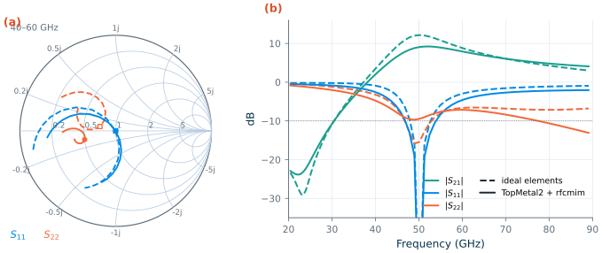
sp: ideal elements (dashed) and TopMetal2 lines with cap_rfcmim (solid), each solved for Eq. (17.2) with RL = 45 Ω. (a) S11 and S22 from 40 to 60 GHz (markers at 50 GHz). (b) |S21|, |S11| and |S22|; dotted: −10 dB.The TopMetal2 amplifier has S21 = 9.07 dB at 50 GHz (peak 9.22 dB at 52.5 GHz), S11 = −62.9 dB and S22 = −9.47 dB, and its S11 stays below −10 dB from 47.9 to 53.7 GHz. Where do 3.1 dB go? At 50 GHz the input network delivers only 55.7 % of its input power to the core (2.55 dB) and the output network 79.8 % (0.98 dB). Chapter 16’s Eq. (16.8) explains it: a network of loaded Q \(Q_n\) built from elements of quality \(Q_L\) loses about \(Q_n/Q_L\) of the power,
\[\eta_{net} \approx 1 - \frac{Q_n}{Q_L}, \qquad Q_{L,\,line} = \frac{\beta}{2\alpha}. \tag{17.3}\]The TopMetal2 line has \(Q_L\) = β/2α ≈ 15 at 50 GHz, and the input network must transform 50 Ω to a core impedance whose Q is 5 to 6 (7.11 − j34.0 Ω in the TopMetal2 version), so it loses 33 to 40 % by Eq. (17.3), close to the 44 % simulated. As Chapter 8 found for the stub match, the loss of a line carrying a standing wave is far higher than its 0.583 dB/mm suggests.
Worked example 17.1 · The output stub
The collector should see \(G_L = 1/45\ \Omega\) = 22.2 mS and a susceptance that cancels the output capacitance. For the TopMetal2 version the solution has \(Y_L\) = 22.2 − j37.6 mS: the network supplies −37.6 mS. A shorted stub of length ℓ has \(Z = jZ_c\tan\beta\ell\), so ℓso = 181 µm (βℓ = 21.0°) gives j18.4 Ω, −54 mS, of which the series line and the DC block cancel the rest. The same stub carries the 27.5 mA collector current from \(V_{CC}\), and its end must be a true RF ground: a supply connection there must be decoupled by a capacitor that is a short at 50 GHz, such as the 20 µm cap_rfcmim of Table 17.1.
17.5 Large-signal performance
The load line
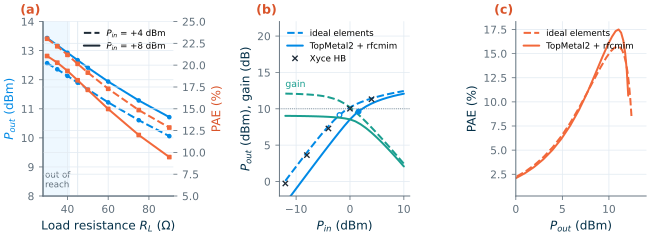
Chapter 16’s load-line argument (Eq. 16.5) sets \(R_L\): with VCC = 1.5 V and a knee near 0.37 V, a +12 dBm collector power needs about 40 Ω. An ideal tuner at the collector, a lossless tank that resonates the 171 fF of output capacitance and shorts the harmonics, gives the curves of Figure 17.4a. The power rises towards low resistance: 13.4 dBm at 30 Ω and 12.7 dBm at 45 Ω for +8 dBm of input; the PAE also peaks at the low end, 21.0 % at 30 Ω against 18.3 % at 45 Ω. Our networks cannot go below 40.9 Ω (37.0 Ω with the pad’s EM value, Chapter 18): the pad in parallel with 50 Ω is 40.9 − j19.3 Ω, and a series element and a collector stub cannot lower the parallel resistance below that series resistance. The design therefore uses RL = 45 Ω, 0.7 dB below the tuner’s best output. A lower load would need a shunt capacitor at the pad and a higher transformation ratio, and so, by Eq. (17.3), more loss. The supply of 1.5 V was chosen for the same reason: at 1.2 V the load-line value would fall to about 22 Ω, out of the networks’ reach.
Simulator
The academy module runs harmonic balance in Xyce. Here a Xyce HB sweep of the ideal-element amplifier (numfreq = 7, stepped source amplitude) converged up to +4 dBm of input; the step to +8 dBm failed. Every large-signal curve below is therefore an ngspice transient of 60 periods at 50 GHz with the powers taken from an FFT of the last 10, as in Chapter 16; where both exist the two agree within 0.36 dB (Figure 17.4b, crosses). The TopMetal2 version, with LTRA lines and cap_rfcmim, runs only in ngspice. Self-heating is on in the HBT model.
Results
Figure 17.4b–c and Table 17.2 give the results. The ideal version has 12.1 dB of small-signal gain and compresses by 1 dB at +9.14 dBm of output (−1.95 dBm input); at +10 dBm of input its output reaches 12.4 dBm, with only 2.44 dB of gain left: that is our Psat. Its PAE peaks at 15.7 % at 10.9 dBm. The TopMetal2 version starts from 9.03 dB, compresses later in input terms and reaches P1dB = +9.62 dBm and Psat = 12.1 dBm; its PAE peaks at 17.5 % at 11.0 dBm. It is higher than with ideal elements because the network presents different harmonic loads (its collector efficiency at the PAE peak is 23.3 % against 18.1 %), while the extra drive power costs little at 2 dB of compressed gain. Both versions draw 27.5–28.2 mA at rest (41.4–42.3 mW) and 36–45 mA at the PAE peak.
Table 17.2. Large-signal results at 50 GHz (ngspice transient + FFT; Psat = output at +10 dBm of available input power).
| Quantity | Ideal elements | TopMetal2 + cap_rfcmim |
|---|---|---|
| Small-signal gain | 12.1 dB | 9.03 dB |
| P1dB (output / input) | 9.14 / −1.95 dBm | 9.62 / 1.59 dBm |
| Psat (gain there) | 12.4 dBm (2.44 dB) | 12.1 dBm (2.07 dB) |
| Peak PAE (at Pout) | 15.7 % (10.9 dBm) | 17.5 % (11.0 dBm) |
| PAE at +10 dBm out | 15.0 % | 16.1 % |
| 2nd / 3rd harmonic at Psat | −8.27 / −18.9 dBc | −10.5 / −13.0 dBc |
| AM-PM up to Psat | −8.78° | −3.35° |
| Collector voltage at Psat (min / max) | 0.434 / 3.65 V | 0.33 / 3.12 V |
Two numbers in the table need attention. The harmonics are strong, −8 to −13 dBc at saturation, because both networks are high-pass at the collector: nothing shorts 100 GHz. A transmitter at 50 GHz would add a harmonic termination or rely on the antenna and the next stage’s selectivity. And the collector swings to 3.12–3.65 V, about twice BVCEO = 1.6 V, though below BVCBO = 4.8 V. As in Chapter 16’s cascode, this is acceptable only because the base is driven from a low impedance at RF, and the average base current stays positive in the simulation (it rises from 58.0 to 307 µA in the TopMetal2 version), so the avalanche current modelled by VBIC does not reverse it. A reliability analysis, and a bias circuit that can sink base current, would come next.
17.6 From ideal elements to layout: what EM adds
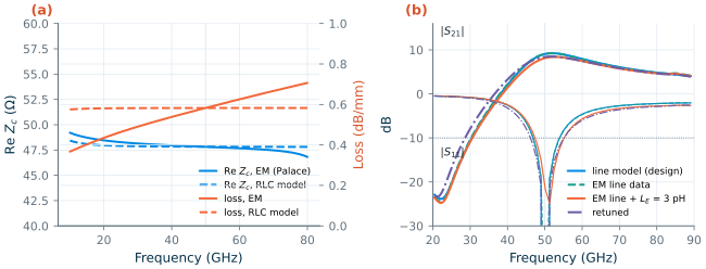
The lines of Section 17.4 already come from EM: Chapter 7 simulated 300 µm and 900 µm TopMetal2 lines in Palace with IHP’s gds2palace flow [198, 197] and extracted the line constants from the pair. Replacing the RLC model by the frequency-dependent EM γ and Zc changes almost nothing (Figure 17.5): the model was fitted at 50 GHz, and between 40 and 60 GHz the EM loss runs from 0.538 to 0.626 dB/mm against a constant 0.583 dB/mm, while Zc stays between 48.0 and 47.7 Ω. S21 at 50 GHz moves from 9.10 to 9.11 dB.
What a real layout adds is everything between the lines: the T-junctions where the stubs branch, the bends, the transition from a line to a MIM capacitor and to the transistor’s contacts, the pad over its shield, and the inductance of the emitter’s path to ground. The academy module handles them as we would: draw the layout, cut the passive part out at the transistor’s terminals, simulate it in openEMS [196] with ports at the cuts (gds2openEMS), and bring the S-parameters back into the circuit simulator, directly or as a vector-fitted SPICE model [3, 172]. Chapter 18 runs that simulation with Palace, and its result is much larger than any single parasitic suggests. First, Figure 17.5b shows the size of the effect of one parasitic that every layout has: 3 pH of emitter inductance, 0.942 Ω at 50 GHz. It lowers S21 from 9.11 to 8.16 dB, raises S11 to −21.6 dB and moves the gain peak to 52.5 GHz. Re-solving the line lengths with it included (ℓi 15.2 µm, ℓsi 221 µm, ℓo 125 µm, ℓso 214 µm) restores the match, but not the gain: 8.42 dB, because emitter degeneration lowers the transistor’s MAG. The laid-out networks cost far more. Drawn with the PDK’s cells to exactly these line lengths and simulated in Palace with second-order elements, they leave 4.82 dB of gain at 50 GHz instead of 9.07 dB, S11 = −10.8 dB and S22 = −7.79 dB, with the gain peak moved to 57.5 GHz (6.87 dB). The landings of the capacitors, their narrow feeds and the junctions add capacitance and inductance, and about twice the loss of the schematic networks; a lumped model of these parasitics does not fit the EM data with physical values, so the design must be retuned with the EM in the loop.
What this means for your design
At 50 GHz the schematic is a first guess. Lay out early, simulate the passive structure, including the transistor’s connections, with EM, and re-solve the match with the result; budget several decibels of gain for what the EM shows (Chapter 18 found 4.3 dB). The order of the academy module, ideal → lines → EM → back-annotate, is the order in which the surprises appear.
17.7 Results and lessons
Table 17.3. The 50 GHz amplifier against its target (typical models, 27 °C, VCC = 1.5 V, 27.5 mA at rest). Fifth column: the networks laid out and simulated with Palace in [Chapter 18](/rfic-design/chapters/18-rf-layout/#tab-18-4). Last column: the cascode redesign of [Section 17.8](#178-a-redesign-with-em-in-the-loop) (VCC = 2.4 V, 23.8 mA), with both networks from full Palace simulations of their layouts.
| Item | Target | Ideal elements | TopMetal2 + cap_rfcmim | After layout (EM, Chapter 18) | Redesign after layout (EM, Section 17.8) |
|---|---|---|---|---|---|
| Small-signal gain at 50 GHz | ≥ 10 dB | 12.2 dB ✓ | 9.07 dB ✗ (8.42 dB with 3 pH emitter inductance, retuned) | 4.82 dB ✗ | 12.4 dB ✓ |
| S11 at 50 GHz | ≤ −10 dB | −59.5 dB ✓ | −62.9 dB ✓ (47.9–53.7 GHz) | −10.8 dB ✓ (marginal) | −14.0 dB ✓ |
| S22 at 50 GHz | ≤ −10 dB | −15.4 dB ✓ | −9.47 dB ✗ (marginal) | −7.79 dB ✗ | −30.6 dB ✓ |
| Stability | μ > 1, 0.1–400 GHz | ✓ (μ = 1 at low frequency, lossless network) | ✓ | ✓ (0.1–160 GHz, the EM band) | ✓ (0.1–160 GHz; μ = 1.001 at 0.5 GHz) |
| P1dB (output) | ≈ +10 dBm | 9.14 dBm ✓ | 9.62 dBm ✓ | 8.07 dBm ✗ | 7.95 dBm ✗ (Psat − 3.5 dB) |
| Psat | ≥ +10 dBm | 12.4 dBm ✓ | 12.1 dBm ✓ | 10.2 dBm ✓ (marginal) | 11.4 dBm ✓ |
| Peak PAE | (reported) | 15.7 % | 17.5 % | 7.44 % | 12.8 % |
The stage meets the power targets with either network, and every target with ideal elements. With TopMetal2 lines and real capacitors it misses the gain target by 0.9 dB, and S22 is marginal, which is expected for a load-line rather than conjugate output match. After layout and EM (Chapter 18) it misses it by 5.2 dB, and S22 is −7.79 dB. The cause is the loss of Eq. (17.3), not the transistor: the stabilized core offers 12.6 dB, and the networks take 3.5 dB. The remedies are the usual ones at millimetre waves: a cascode, whose low S12 needs less stabilizing loss and gives more MAG; a driver stage in front; or a lower-Q input match through a larger device or a stabilization network with less reactance. The +12 dBm and 17.5 % PAE of the power stage are set by the supply, the load line and the transistor, and they survive the schematic’s real lines and capacitors, but not the laid-out networks: the collector then sees 31.2 Ω instead of 45 Ω and the output network passes 48 % of the power instead of 80 %, so Psat falls to 10.2 dBm and the peak PAE to 7.44 %. After layout these remedies are necessary rather than optional, and the networks must be designed with the EM in the loop. Section 17.8 does both. For comparison, Pfeiffer and Goren’s 60 GHz SiGe PA reached +20 dBm with a multi-stage cascode design and on-chip power combining [171].
17.8 A redesign with EM in the loop
This section designs the amplifier again, in the order a second pass at millimetre waves should follow. First, the core gets more gain, so that the networks may lose some. Second, the networks are designed from small EM-simulated pieces, so that the design already contains what the layout adds. Third, each finished network is simulated once in Palace, to check the result.
A cascode core
The gain comes from a cascode. Q1 is the common-emitter transistor of Section 17.2 (four npn13G2 with Nx = 4, VBE = 0.90 V). Above it, Q2 is a common-base transistor of the same size, whose base is held at VB2 = 1.8 V through 13 Ω and decoupled by four 10 µm cap_rfcmim. With VCC = 2.4 V the pair draws 23.8 mA, and Q1 sits at VCE = 0.91 V. Q2 isolates Q1’s collector from the output: S12 at 50 GHz falls from −21.2 dB for the single stage to −47.5 dB, and \(\vert S_{21}\vert\) between 50 Ω ports rises from 9.55 to 17.8 dB.
Breakdown sets the supply, as in Chapter 16. At rest Q2 has VCE = 1.49 V, below BVCEO = 1.6 V. At full drive its collector swings to 4.91 V, so vCB of Q2 peaks at 3.1 V, below BVCBO = 4.8 V, while vCE goes well past BVCEO. That is acceptable only because Q2’s base is held at a low impedance (Section 16.6). With the ideal tuner of Figure 17.4a, the cascode delivers up to 14.2 dBm into 50 Ω at 2.4 V, with 29 % PAE, so the collector should again see about 50 Ω.
Rst‖Cst of Section 17.3 stays at the base, but the stabilized cascode is still only conditionally stable (K = 0.853 at 50 GHz, μ down to 0.936 near 87 GHz). The collector needs a second element, and the reason is S22 as much as stability. A load-line match leaves the transistor’s own output resistance Ro unmatched. The single stage has a low Ro, and its S22 came out near −9.5 dB. The cascode’s Ro is 444 Ω, and the same match gives S22 = −3.1 dB. If the network transforms the load RL to the collector without loss, the reflection at the output pad is the mismatch at the collector, so
\[\vert S_{22}\vert = \left\vert\frac{R_o - R_L}{R_o + R_L}\right\vert \le 0.316 \quad\Rightarrow\quad \frac{R_L}{1.92} \le R_o \le 1.92\,R_L. \tag{17.4}\]A resistor Rp from the collector to ground sets Ro ≈ Rp and takes the fraction RL/(RL + Rp) of the collector power: at least 34 % (1.8 dB) for S22 = −10 dB. The design uses Rp = 150 Ω in series with a 20 µm cap_rfcmim that blocks the DC, and lets the output network present RL = 75 Ω. The collector still sees 150 Ω ‖ 75 Ω = 50 Ω, and a third of the power goes into Rp. Rp also damps the output: the core now has K = 4.14 and an MAG of 18.2 dB at 50 GHz, μ ≥ 1.10 from 20 to 400 GHz, and Ro = 113 Ω. The alternative, resistive feedback from the collector to the base, reached S22 = −10.4 dB with 300 Ω, but left only 10.2 dB of gain even with circuit models of the networks.
EM-calibrated building blocks
Chapter 18 could not fit lumped parasitics to a whole network. Here the networks are cut into a few pieces instead. Each piece is simulated once in Palace (second order, 4 µm mesh, 0.01–160 GHz), with its ports at the ends of 16 µm arms of the Chapter 7 microstrip:
- BLK, the DC block: a 20 µm cap_rfcmim with 16 µm feeds (the PDK’s default is 3 µm, and Sections 17.4 and 18.6 used 2 µm), the landings down to its plates, and an arm on each side;
- TEE, a T-junction of three 16 µm lines;
- DEC, the decoupled end of a stub: an arm, a landing, a cap_rfcmim whose bottom plate is stacked down to the Metal1 ground, and the 8 µm bias or supply feed;
- the 80 µm GSG pad of Chapter 18 (37.2 fF). A combined pad and DC-block piece was tried first, but gmsh lost its ports at every mesh size.
Each piece takes 1 to 10 minutes on the laptop. The networks of Figure 17.1 are then built from these blocks and Chapter 7’s EM line data by nodal analysis in Python, and Eq. (17.2) is solved for the four line lengths as before (Table 17.4).
Table 17.4. The building blocks at 50 GHz: Palace (order 2) against the circuit models a schematic design would use. Impedances of BLK are its series impedance with the arms removed; impedances of DEC are seen at the end of its arm.
| Block | Circuit model | EM |
|---|---|---|
| TEE, S21 | 0.665 ∠ −5.6° (ideal node) | 0.664 ∠ −6.6° |
| BLK, 20 µm, 16 µm feeds | 0.95 + j1.93 Ω | 1.81 − j0.82 Ω |
| DEC, 20 µm capacitor, supply on the feed | 0.15 + j2.32 Ω (ideal short) | 6.61 + j2.16 Ω |
| DEC, 20 µm capacitor, RB on the feed | 1.01 + j2.70 Ω | 1.89 − j0.29 Ω |
| DEC, 30 µm capacitor, supply on the feed | 0.15 + j2.32 Ω (ideal short) | 1.63 + j3.30 Ω |
| DEC, 30 µm capacitor, RB on the feed | 1.33 + j7.00 Ω | 1.96 + j2.78 Ω |
The T-junction behaves like an ideal node, with the lines measured from its centre. The DC block has twice the model’s resistance and is still capacitive at 50 GHz, which the design simply absorbs. The surprise is the stub end. With a 20 µm capacitor and wide feeds, the capacitor is still capacitive at 50 GHz, and the short supply feed, an inductance to the ideal supply, resonates with it in parallel. The stub end, which should be a short, is 6.61 Ω, and at the end of the output stub it would take about 40 % of the output power. This is the kind of loss Chapter 18 found but could not attribute; here a block simulation of four minutes isolates it. A 30 µm capacitor (1.36 pF) has its series resonance below 50 GHz, so it is inductive there and cannot resonate with the feed. The stub end becomes 1.63 + j3.30 Ω, and the design uses it at both stubs.
Layout, DRC and the EM check
On the EM blocks the design gives ℓi = 107 µm, ℓsi = 117 µm, ℓo = 179 µm and ℓso = 175 µm, with S21 = 13.1 dB, S22 = −17.4 dB and μ ≥ 1.001. The same design on the circuit models of the blocks gives 143, 70.7, 162 and 202 µm and 14.9 dB: the lengths change by up to 47 µm, and the EM blocks cost 1.8 dB that a schematic design would not see. The two networks are drawn with Chapter 18’s layout code as exactly this cascade of blocks and lines (tools/em/ch17_pa/ch17_layout.py). The DC block now sits one arm from the pad, which also clears the Pad.d1R spacing Chapter 18 violated. The PDK’s KLayout deck reports only the two Slt.c.M1 slit regions per network that Chapter 18 also left. Each network is then simulated once in Palace, second order: the input network in 56 minutes (7 µm mesh) and the output network in 65 minutes (7.5 µm, after gmsh lost the ports at 6 µm).
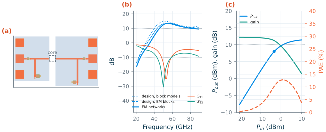
Figure 17.6 and the last column of Table 17.3 give the result. With both networks from the full EM, the amplifier has 12.4 dB of gain at 50 GHz (peak 13.5 dB at 55 GHz, 3 dB band 45.7–89.1 GHz), S11 = −14.0 dB and S22 = −30.6 dB, and μ > 1 from 0.1 to 160 GHz. Its minimum, 1.001 at 0.5 GHz, is the lossless DC blocks of Section 17.3 again. The full EM costs 0.7 dB more than the EM blocks predicted, not the 4.3 dB of Chapter 18, and moves the input match a few gigahertz up. What the blocks miss is small: the coupling between neighbouring pieces and the field at the joints where two block ports meet. The ngspice version, with the networks vector-fitted to 130 GHz, agrees within 0.3 dB (12.7 dB, S11 = −14.7 dB, S22 = −27.3 dB). Fitted to 160 GHz, the output network’s model came out slightly active, with a largest singular value of 1.11; scaling it down to passive, as Chapter 18 did, would have cost about 1 dB.
In the transient sweep the gain starts at 12.2 dB. The output reaches Psat = 11.4 dBm at +10 dBm of drive, and the PAE peaks at 12.8 % at 10.0 dBm. The gain, S11, S22, stability and Psat targets are now met after layout and EM. Two numbers are worse than in the first design’s schematic. P1dB is 7.95 dBm, 2 dB short of the ≈ +10 dBm of Table 17.3: the cascode compresses gradually, 3.5 dB below Psat. And the peak PAE stays below the schematic’s 17.5 %, although it is well above the 7.44 % of the first design after layout. Rp takes a third of the collector power, and the 2.4 V supply raises the DC power by about 40 % for a similar output. The second harmonic is strong, −6.6 dBc at Psat, because nothing at the collector shorts 100 GHz.
A next iteration would win these back at the output. One option is a harmonic short at the collector, such as a λ/4 stub at 100 GHz, which sharpens the compression and raises the PAE. Another is to meet S22 with a balanced pair of amplifiers between 90° hybrids instead of Rp, which removes the 1.8 dB. A third is an output network designed for a lower collector resistance, for more P1dB. Each would again be designed on EM blocks and checked with one EM run per network.
What this means for your design
EM in the loop does not mean EM in every iteration. Simulate each kind of piece once, with its ports where the circuit cuts it, design the network on those S-parameters, and spend the long EM run on the finished layout only. Here four block runs of 1 to 10 minutes, and two network runs of about an hour, turned a design that lost 4.3 dB after layout into one that lost 0.7 dB.
Try it · The 50 GHz amplifier script
Every number in this chapter comes from
tools/figs/ch17_mmwave_pa.py(python3 tools/figs/ch17_mmwave_pa.py device matchruns in seconds;largeruns the transients and the Xyce check in about four minutes). Three experiments: (1) ChangeRST, CSTto 70 Ω and 130 fF and re-rundevice match --resim: the TopMetal2 gain rises, but what happens to μ of the complete amplifier? (2) SetW_BLK = 20(a self-resonant DC block) and explain, with Section 17.5, why the output network can no longer reach 45 Ω. (3) Inem(), raiseLEto 8 pH and compare the retuned gain with the 8.42 dB of Figure 17.5. Section 17.8 comes fromtools/figs/_ch17_redesign.py(core,design,verify,fig) and the layouts and Palace runs intools/em/ch17_pa/: setOPT["rp"]to 0 andRL_DESto 50 indesignand see S22 collapse.
- At 50 GHz a tenth of a wavelength on TopMetal2 is 310 µm, a 30 fF pad is −j106 Ω (the EM pad of Chapter 18, 37.7 fF, is −j84.4 Ω), a 20 µm MIM capacitor is self-resonant and 3 pH of emitter lead is about 1 Ω: all of them belong in the design.
- Four npn13G2 (Nx = 4) at 27.5 mA have fT = 344 GHz, fmax = 455 GHz and an MSG of 15.4 dB at 50 GHz, but K = 0.387; a series R‖C (100 Ω, 100 fF) and a resistive bias feed make the amplifier stable from 0.1 to 400 GHz for 2.8 dB of gain.
- Stub-and-line networks double as bias feeds. With ideal elements the stage has 12.2 dB of gain; with TopMetal2 lines (Q ≈ 15) and cap_rfcmim it has 9.07 dB, because a network of Qn loses about Qn/QL of the power (Eq. 17.3).
- The load line sets RL = 45 Ω at VCC = 1.5 V; the stage reaches P1dB ≈ +9.6 dBm, Psat ≈ +12 dBm and 17.5 % peak PAE in ngspice transients (Xyce HB converged only to +4 dBm of drive), with a collector peak of about twice BVCEO.
- A cascode redesign (Section 17.8) meets the gain, match, stability and Psat targets after layout: 12.4 dB, S11 = −14.0 dB, S22 = −30.6 dB, Psat = 11.4 dBm, 12.8 % PAE; its P1dB, 7.95 dBm, stays 2 dB short. Its networks were designed on EM-simulated blocks; one of them showed a stub-end capacitor resonating with its supply feed, which a larger capacitor removed. A load-line match of a cascode needs a resistor at the collector to meet S22 (Eq. 17.4), at a cost of at least 1.8 dB of output power.
- EM line data confirm the line model; junctions, pads and the emitter connection are what EM must add, and the match must be re-solved afterwards. With the networks laid out and simulated in Palace (Chapter 18), the gain at 50 GHz falls to 4.82 dB and Psat to 10.2 dBm: the EM belongs in the design loop.
Further reading
- IHP Analog Academy, module 2 [3]: the 50 GHz MPA in SG13G2 step by step in Qucs-S, ngspice, Xyce and openEMS, the workflow this chapter follows.
- S. P. Voinigescu, High-Frequency Integrated Circuits [10]: SiGe HBT sizing, biasing and millimetre-wave amplifier and PA design.
- S. C. Cripps, RF Power Amplifiers for Wireless Communications [13]: the load-line match used in Section 17.5.
- U. R. Pfeiffer and D. Goren [171]: a fully integrated 60 GHz SiGe PA with +20 dBm, for what a multi-stage design reaches.
- IHP’s openEMS and Palace flows [198, 196, 197], and B. Gustavsen and A. Semlyen [172] on vector fitting, for bringing EM results back into the circuit simulator.