Lab 2
RF Transistors
Measure the two transistors of the course the way an RF designer does: from their S-parameters and noise parameters, at many bias points, with scikit-rf turning every Touchstone file into fT, fmax, gains, stability factors and noise figures.
- Simulate a transistor as a two-port with ngspice
spand the noise flag, and sweep its bias from Python.- Extract fT and fmax from the current gain h21 and Mason’s U with scikit-rf, by extrapolation and by direct crossing, and explain the difference.
- Read MAG or MSG, K and μ from a
Network, and explain why a transistor is potentially unstable at low frequencies.- Find the minimum noise figure and the optimum source impedance against bias and frequency.
- Relate the SG13G2 RF model’s gate resistance to the layout: fingers and cells.
Contents
| Lab 2 at a glance | |
|---|---|
| Goal | fT, fmax, MAG/MSG, K, μ, NFmin and Zopt of the SG13G2 RF nMOS and the npn13G2 HBT from ngspice sp, analysed with scikit-rf, against Chapter 6’s Table 6.2. |
| Chapters | Chapter 6 (Sections 6.1–6.6, Worked examples 6.1 and 6.2, Figure 6.4, Table 6.2); stability and gains from Chapter 3 (Sections 3.6–3.7) |
| Time | 2–3 hours |
| Files | tools/labs/lab2/: nmos_sp.cir, hbt_sp.cir, transistors.py |
| Run time | transistors.py about 10 s for all three parts (56 ngspice runs) |
Run every command in tools/labs/lab2, inside the container or from your computer with ../common/iic.sh in front of it.
Hand calculation
The reference nMOS of Chapter 6 is 20 µm wide, drawn as two cells (\(m\) = 2) of five 2 µm fingers at L = 0.13 µm, with IHP’s RF model (rfmode=1), biased at \(V_{GS}\) = 0.95 V and \(V_{DS}\) = 0.6 V.
- Gate resistance. With Eq. (6.6) (\(R_{SHG}\) = 3 Ω/□, \(X_{GW}\) = 0.1 µm, \(R_{INT}\) = 13.0 Ω µm², \(R_{GO}\) = 40 Ω per cell), compute \(R_g\) for the reference device and for the same 20 µm drawn as one cell of ten fingers and as ten cells of one finger.
- fT and fmax. Worked example 6.1 reads \(g_m\) = 13.8 mS, \(g_{ds}\) = 1.19 mS, \(C_{gg}\) = 31.8 fF and \(C_{gd}\) = 11.0 fF from the Y-parameters at 1 GHz. Compute \(f_T\) with Eq. (6.1) and \(f_{max}\) with Eq. (6.4), keeping the \(g_{ds}R_g\) term.
- Maximum stable gain. Where \(K\) < 1 the best gain is the MSG, \(\vert S_{21}/S_{12}\vert = \vert y_{21}/y_{12}\vert\). With \(y_{21} \approx g_m\) and \(y_{12} \approx -j\omega C_{gd}\), estimate it at 2.4 GHz in dB.
Steps
-
The testbench. Open
nmos_sp.cir. Port 1 drives the gate and port 2 the drain through ideal bias tees (1 F, 1 H), as in Chapter 6; the first.paramline holds the bias.sp dec 20 1e8 1e11 1sweeps 0.1–100 GHz with the noise flag,wrs2pwrites the S-parameters andwrdatathe noise parameters.hbt_sp.cirdoes the same for annpn13G2with \(N_x\) = 4 at \(V_{CE}\) = 1.2 V. Run one by hand:ngspice -b nmos_sp.cirprints \(I_D\) = 3.738 mA. -
One bias point of each device. Run
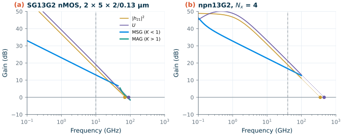
python3 transistors.py one. For each device it reads the files into a scikit-rfNetworkwith the noise parameters attached (labkit.read_sp) and computes:y = n.y h21 = abs(y[:, 1, 0] / y[:, 0, 0]) # short-circuit current gain U = n.unilateral_gain # Mason's U G = n.max_gain # MAG where K > 1, MSG where K < 1 K = n.stability # Rollett's K n.nfmin_db, n.z_opt, n.rn # noise parameters\(f_T\) and \(f_{max}\) are extrapolated at −20 dB per decade from a spot frequency, 10 GHz for the nMOS and 40 GHz for the HBT, as Chapter 6 and IHP’s process specification do (Eq. 6.2); the script also reports where \(\vert h_{21}\vert\) and \(U\) actually cross one. It prints the small-signal values of your hand calculation, from the Y-parameters at 1 GHz, and draws Figure L2.1.
- Bias sweeps. Run
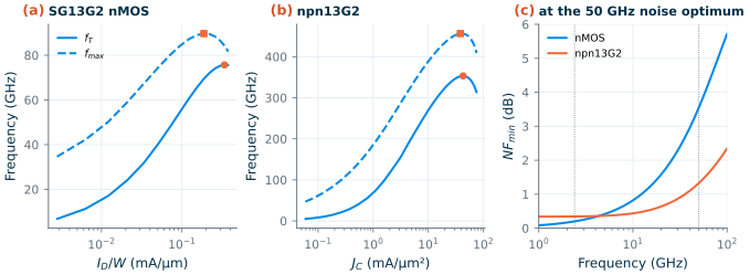
python3 transistors.py sweep. It writes a copy of each netlist per bias point intoout/sweep/(only the.paramline and the output names change) and runs them: the nMOS at \(V_{GS}\) = 0.30–1.20 V in 50 mV steps and the HBT at \(V_{BE}\) = 0.70–1.00 V in 10 mV steps, the grids of Chapter 6. From eachNetworkit takes \(f_T\), \(f_{max}\) and the noise parameters at 2.4 and 50 GHz, then finds the peaks of \(f_T\) and \(f_{max}\) and the bias of minimum \(NF_{min}\) at each frequency. It counts a bias point for the noise minimum only if the device still amplifies there (\(f_T\) above half the frequency and \(U\) above 3 dB): at very low currents the device is a nearly lossless capacitor and the computed \(NF_{min}\) falls towards 0 dB without meaning anything. Figure L2.2 shows the result.
- Fingers and cells. Run
python3 transistors.py cells. It replaces the device line to draw the same 20 µm of 2 µm fingers as 1, 2, 5 and 10 cells, all at \(V_{GS}\) = 0.95 V, and prints the input resistance \(\mathrm{Re}(1/y_{11})\) at 10 GHz next to Eq. (6.6), with \(f_T\), \(f_{max}\) and \(C_{gg}\): Chapter 6’s Figure 6.4 in four rows.
Checkpoint
Table L2.1. One bias point (step 2). nMOS: VGS = 0.95 V, VDS = 0.6 V; npn13G2: VBE = 0.93 V, VCE = 1.2 V. Tolerance ±1 in the last digit; hand values within 2 % of the simulation.
| Quantity | Lab 2 | Chapter 6 |
|---|---|---|
| nMOS: \(I_D\); \(g_m\), \(g_{ds}\), \(C_{gg}\), \(C_{gd}\) at 1 GHz | 3.74 mA; 13.8 mS, 1.19 mS, 31.8 fF, 11.0 fF | 3.74 mA; 13.8 mS, 1.19 mS, 31.8 fF, 11.0 fF |
| nMOS: \(f_T\) hand (Eq. 6.1) / extrapolated / direct crossing | 69.2 / 69.5 / 78.4 GHz | 69.2 / 69.5 GHz |
| nMOS: \(f_{max}\) hand (Eq. 6.4) / extrapolated / direct crossing | 88.8 / 89.7 / 81.8 GHz | 88.8 / 89.7 GHz |
| nMOS: \(R_g\) (Eq. 6.6) / \(\mathrm{Re}(1/y_{11})\) at 10 GHz | 25.5 / 26.5 Ω | 25.5 / 26.5 Ω |
| nMOS at 2.4 GHz: MSG (hand ≈ \(g_m/\omega C_{gd}\): 19.2 dB), \(K\), \(\mu\) | 19.2 dB, 0.045, 0.059 | |
| nMOS at 50 GHz: \(K\), \(\mu\); MAG / MSG | 1.01, 1.007; 5.59 / 6.24 dB | |
| npn13G2: \(I_C\), \(\beta\) | 9.60 mA (38.1 mA/µm²), 394 | |
| npn13G2: \(f_T\), \(f_{max}\) (extrapolated from 40 GHz) | 352, 456 GHz | 353, 456 GHz at the peaks |
| npn13G2 at 2.4 / 50 GHz: MSG; \(K\) | 28.9 / 15.7 dB; 0.018 / 0.40 |
Table L2.2. Bias sweeps (step 3) against Chapter 6's Table 6.2 (current densities in mA/µm for the nMOS and mA/µm² of drawn emitter area for the HBT; tolerance ±1 in the last digit).
| Quantity | nMOS: Lab 2 | Table 6.2 | npn13G2: Lab 2 | Table 6.2 |
|---|---|---|---|---|
| Peak \(f_T\) (at J) | 75.7 GHz (0.336) | 75.7 GHz (0.336) | 353 GHz (42.8) | 353 GHz (42.8) |
| Peak \(f_{max}\) (at J) | 89.7 GHz (0.187) | 89.7 GHz (0.187) | 456 GHz (38.1) | 456 GHz (38.1) |
| Minimum \(NF_{min}\) at 2.4 GHz (at J) | 0.200 dB (0.153) | 0.200 dB (0.153) | 0.224 dB (0.552) | 0.224 dB (0.552) |
| Minimum \(NF_{min}\) at 50 GHz (at J) | 3.55 dB (0.123) | 3.55 dB (0.123) | 1.33 dB (4.28) | 1.33 dB (4.28) |
| At the 50 GHz optimum: \(\Gamma_{opt}\) at 2.4 / 50 GHz | 0.981∠2.07° / 0.670∠38.7° | 0.981∠2.07° / 0.670∠38.7° | 0.931∠1.04° / 0.746∠21.6° | |
| \(Z_{opt}\) at 2.4 / 50 GHz | 1160 + j2140 / 68.3 + j104 Ω | 1160 + j2140 / 68.3 + j104 Ω | 1320 + j338 / 131 + j162 Ω | 1320 + j338 / 131 + j162 Ω |
| \(R_n\) at 2.4 / 50 GHz | 118 / 104 Ω | 118 / 104 Ω | 55.9 / 55.2 Ω | 55.9 / 55.2 Ω |
Table L2.3. The same 20 µm nMOS drawn as cells of 2 µm fingers (step 4), VGS = 0.95 V. Chapter 6's values (Figure 6.4 and its text) are identical.
| Cells × fingers | Re(1/y11) at 10 GHz | Eq. (6.6) | Cgg | fT | fmax |
|---|---|---|---|---|---|
| 1 × 10 | 46.6 Ω | 45.5 Ω | 31.6 fF | 70.0 GHz | 66.5 GHz |
| 2 × 5 (reference) | 26.5 Ω | 25.5 Ω | 31.8 fF | 69.5 GHz | 89.7 GHz |
| 5 × 2 | 15.5 Ω | 13.5 Ω | 41.8 fF | 52.8 GHz | 101 GHz |
| 10 × 1 | 11.4 Ω | 9.51 Ω | 42.8 fF | 51.6 GHz | 117 GHz |
Every value that Chapter 6 quotes is reproduced, now through scikit-rf instead of the chapter’s own helpers: the peaks, the noise optima and the optimum source impedances fall on the same bias points of the same grids. Your hand calculations should give \(R_g\) = 45.5, 25.5 and 9.51 Ω, \(f_T\) = 69.2 GHz, \(f_{max}\) = 88.8 GHz and an MSG of 13.8 mS/(2π × 2.4 GHz × 11.0 fF) = 83, or 19.2 dB.
Questions
- At 2.4 GHz the nMOS has \(K\) = 0.045, and at 50 GHz \(K\) = 1.01. Why is a transistor more likely to be unconditionally stable near its \(f_{max}\) than at a tenth of it? What does the MSG’s slope of 10 dB per decade in Figure L2.1 tell you about \(y_{12}\)?
- The direct crossing of \(\vert h_{21}\vert\) gives 78.4 GHz, 13 % above the extrapolated 69.5 GHz, while for \(U\) the crossing is below the extrapolation. Which current makes \(\vert h_{21}\vert\) level off above \(f_T\) (Section 6.1)? Which of the two numbers would you put in a datasheet?
- Ten single-finger cells reach 117 GHz of \(f_{max}\) but only 51.6 GHz of \(f_T\). Which two terms of the RF model change between the 2 × 5 and the 10 × 1 layout, and which way does each push?
- The HBT’s \(NF_{min}\) at 2.4 GHz is 1.12 dB at \(V_{BE}\) = 0.93 V but 0.224 dB at its noise optimum, 70 times less current. Which noise sources grow with the collector current, and why is a bipolar’s noise optimum at such a low current density?
- At the 50 GHz optimum, \(Z_{opt}\) of the 20 µm nMOS is 68.3 + j104 Ω. How wide must the device be for \(\mathrm{Re}(Z_{opt})\) = 50 Ω, and what happens to \(R_n\) (Worked example 6.4)?
Extension
Rerun the nMOS sweep at \(V_{DS}\) = \(V_{DD}\) = 1.2 V: in part_sweep of transistors.py change vds=0.6 to vds=1.2 (and the output tag, so that both sweeps stay in out/sweep/). Compare the peaks with the second row of Table 6.2 (89.5 GHz at 0.424 mA/µm; Section 6.3 gives 109 GHz of \(f_{max}\) at 0.335 mA/µm). Then add a third device: copy nmos_sp.cir to hv_sp.cir with the 3.3 V sg13_hv_nmos (L = 0.45 µm, the library cornerMOShv.lib (section mos_tt) next to cornerMOSlv.lib, \(V_{DS}\) = 1.65 V, \(V_{GS}\) from 0.5 to 3.3 V) and find its peak \(f_T\) and \(f_{max}\); Table 6.2 gives 16.0 GHz and 71.6 GHz. Which block of the course radio, if any, could use it?