Chapter 19
The Complete Transceiver
Chapter 5 turned Bluetooth Low Energy into a budget, and ten chapters designed the blocks to it. This chapter puts them back together. It checks every block against its target, rebuilds the receive and transmit chains from the simulated numbers, runs the behavioural receiver of Chapter 5 with them, and then looks at what a block-by-block design cannot see: the PA pulling the VCO, spurs, leakage, the calibrations that hold it all together, and what happens when the radio shares a phone with an LTE transmitter. It ends with where to take the design next.
- Compare designed blocks with a link budget, and judge a margin by how it was obtained: simulation, hand analysis or assumption.
- Cascade gain, noise figure, IIP3 and IIP2 from the designed blocks, find the noise and distortion shares, and test how far a doubtful number may move before the system fails.
- Run a behavioural receiver with the designed numbers and read the BLE compliance margins, including carrier offset, ADC resolution, blocking and intermodulation.
- Check a transmitter against its output power, efficiency, emission limits and modulation accuracy, and estimate VCO pulling, reference spurs and LO leakage with simple models.
- Explain the calibrations a radio of this kind needs, and the coexistence problem of a radio inside a smartphone.
Contents
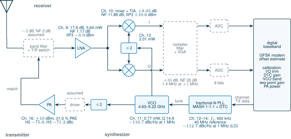
Figure 19.1 is the course radio as the block chapters left it. Blue blocks were designed and simulated in SG13G2 (Chapters 9–16); grey dashed blocks were never designed in the course and enter this chapter as stated assumptions, exactly as Chapter 5 allocated them: the band filter and T/R switch, the complex channel filter and VGA, the ADCs and the PA’s driver. Every number in this chapter comes from tools/figs/ch19_transceiver.py, which reads the block chapters’ result files (tools/figs/ch09_numbers.json to ch16_numbers.json), imports Chapter 5’s receiver, Chapter 12’s loop and Chapter 14’s synthesizer budget, and runs no new transistor-level simulation.
Further learning · Open-SERDES Tutorial
A radio is one kind of transceiver; a wireline serial link is another, built from the same SG13G2 HBTs and CMOS. BRICD’s open tutorial Designing a Serial Link from Scratch designs a 5 Gb/s SerDes in IHP SG13G2, and its Part III · Transceiver Circuits turns the link model into transistors: the serializer and output driver on the transmit side, and the termination, front-end and samplers on the receive side. Its later chapters on jitter, PLL clock generation and clock and data recovery continue Chapters 12–15 of this course in a wireline setting.
19.1 From the link budget to block specifications
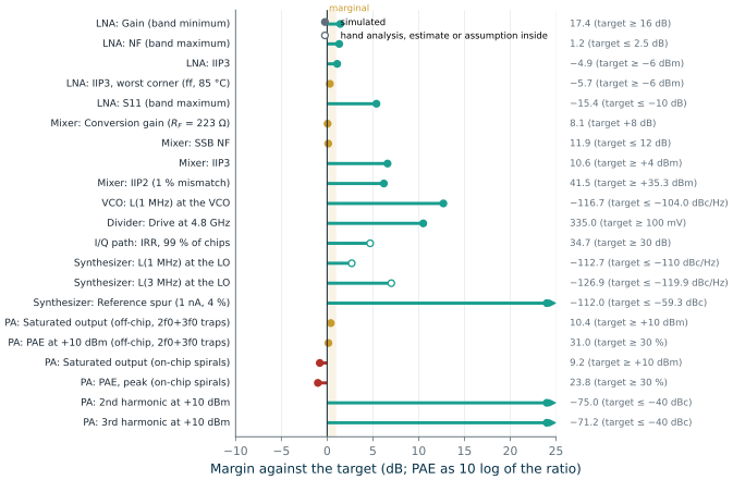
Table 5.3 gave each block of the receiver a gain, a noise figure (NF) and an input third-order intercept (IIP3), and the synthesizer a phase-noise target, so that the cascade would reach an NF of 6.06 dB, an IIP3 of −12.7 dBm and a sensitivity of −95.6 dBm, with 5.6 dB to spare against the course’s −90 dBm. The course radio’s specification added the transmitter: +10 dBm into 50 Ω, a power-added efficiency (PAE) of at least 30 %, and harmonics below −40 dBc. Table 19.1 puts the designed blocks next to those targets.
Table 19.1. The designed blocks against Table 5.3 and the course radio (tt, 27 °C unless stated). Margin in dB; for PAE, 10 log of the ratio. "Hand" and "assumed" mark numbers that no simulation in the course produced.
| Block | Item | Target | Designed | Margin | How obtained |
|---|---|---|---|---|---|
| LNA (Ch. 9) | gain, band minimum | ≥ 16 dB | 17.43 dB | +1.43 | ngspice S-parameters |
| NF, band maximum | ≤ 2.5 dB | 1.18 dB | +1.32 | ngspice noise | |
| IIP3 | ≥ −6 dBm | −4.9 dBm | +1.1 | Xyce harmonic balance | |
| IIP3, worst corner (ff, 85 °C) | ≥ −6 dBm | −5.7 dBm | +0.3 | Xyce harmonic balance | |
| S11, band maximum | ≤ −10 dB | −15.39 dB | +5.39 | ngspice S-parameters (−13.5 dB with Chapter 18’s EM pad) | |
| Mixer + TIA (Ch. 10), transistor-level OTA, RF = 223 Ω | conversion gain | +8 dB | +8.05 dB | +0.05 | Xyce transient, PSP switches and OTAs (behavioural op-amp at 220 Ω: +8.02 dB) |
| SSB NF | ≤ 12 dB | 11.88 dB | +0.12 | periodic small-signal analysis with the OTA’s simulated admittance and noise, 0.5–1.5 MHz average (behavioural op-amp: 11.25 dB) | |
| IIP3 | ≥ +4 dBm | +10.6 dBm | +6.6 | Xyce two-tone with the OTAs | |
| IIP2, 1 % switch mismatch | ≥ +35.3 dBm | ≥ +41.5 dBm | +6.2 | Xyce two-tone with the OTAs, lowest value from −22 to −10 dBm (behavioural op-amp: +56.0 dBm) | |
| VCO (Ch. 11) | L(1 MHz) at the VCO | ≤ −104.0 dBc/Hz | −116.7 dBc/Hz | +12.7 | ISF and frozen noise of every source (equivalent F = 3.71) |
| coverage of 4.802–4.962 GHz | with margin | 4.633–5.224 GHz (tt) | 1.0 % (fast corner, lower edge) | transients, three corners | |
| Divider (Ch. 13) | drive at 4.8 GHz | ≥ 100 mV | 335 mV | +10.5 | transient |
| I/Q path (Ch. 13, 10) | IRR, 99 % of chips | ≥ 30 dB | 34.7 dB | +4.7 | Monte Carlo, Section 19.2 (baseband assumed) |
| Synthesizer (Ch. 12–14) | L(1 MHz) at the LO | ≤ −110 dBc/Hz | −112.7 dBc/Hz | +2.7 | linear loop model with the simulated VCO and the modelled, calibrated DTC (impairments assumed) |
| L(3 MHz) at the LO | ≤ −119.9 dBc/Hz | −126.9 dBc/Hz | +7.0 | the same | |
| reference spur (1 nA, 4 % mismatch) | ≤ −59.3 dBc | −112 dBc | +52.7 | Fourier series of the pump current | |
| PA (Ch. 16), off-chip Q = 40, 2f0 and 3f0 traps | saturated output | ≥ +10 dBm | +10.4 dBm | +0.4 | ngspice transient |
| PAE at +10 dBm | ≥ 30 % | 31.0 % | +0.14 | ngspice transient | |
| 2nd harmonic at +10 dBm | ≤ −40 dBc | −75.0 dBc | +35.0 | ngspice transient | |
| 3rd harmonic at +10 dBm | ≤ −40 dBc | −71.2 dBc | +31.2 | ngspice transient | |
| PA, on-chip spirals | saturated output, peak PAE | ≥ +10 dBm, ≥ 30 % | +9.2 dBm, 23.8 % | −0.8, −1.0 (fail) | ngspice transient |
Figure 19.2 shows the same margins at a glance. Of the 22 numbers, two fail and five are marginal (less than 1 dB). Both failures belong to the on-chip PA, which Chapter 16 already reported: with the Chapter 7 spirals its output network loses 29 % of the power. Off chip, with Q = 40 inductors and the harmonic traps that Chapter 16 added (3f0 at the collector, 2f0 at the output), the PA meets its specification, if only just: 31.0 % PAE against 30 %. All five marginal numbers are simulated, so the margins are small but real: the LNA’s IIP3 at the fast corner and 85 °C, the PA’s saturated power and PAE, and the mixer’s gain and noise figure, which Chapter 10 simulates with a transistor-level OTA in both TIAs and RF = 223 Ω. The OTA’s noise takes the mixer from the behavioural op-amp’s 11.25 dB to 11.88 dB, 0.12 dB inside its 12 dB budget. That is the number to watch, and Section 19.2 asks how far it may move.
What this means for your design
A margin is only as good as the way it was obtained. The synthesizer’s 2.7 dB at 1 MHz looks comfortable, and its VCO is now simulated with every noise source (Chapter 11), but its DTC is a behavioural model whose gain error, INL and jitter are assumed sizes (Chapter 14); the LNA’s 0.3 dB of IIP3 margin at the worst corner looks thin, but it is a simulated corner. When you sign off a block, record next to each number how it was obtained, and spend the next verification effort where an unsimulated number sits close to its limit.
19.2 The receive chain
The cascade with the designed numbers
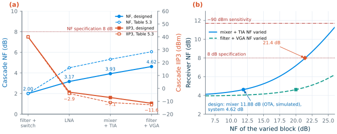
The designed blocks do not match the budget one for one. The LNA has 1.6 dB more gain and 1.3 dB less noise than allocated; the mixer, with its transistor-level OTA, has 0.12 dB less noise and 6.6 dB more IIP3. The cascade moves accordingly. With the gains, NFs and IIP3s of Table 19.2, the Friis formula (Eq. (4.11)) and the cascaded-IIP3 formula of Chapter 4 give an NF of 4.62 dB and an IIP3 of −11.6 dBm, against 6.06 dB and −12.7 dBm in the budget. By Eq. (4.12), with SNRmin = 12.3 dB in 1 MHz, the sensitivity is −97.1 dBm: 7.1 dB better than the course’s −90 dBm and 27.1 dB better than BLE’s −70 dBm.
Which block should be improved first? The noise share of block \(k\) is its term in the Friis sum relative to the whole:
Key equation · Noise share of a block in a cascade
\[s_1 = \frac{F_1}{F}, \qquad s_k = \frac{F_k - 1}{F\,G_1G_2\cdots G_{k-1}} \quad (k > 1), \qquad \sum_k s_k = 1 \tag{19.1}\]\(F\) is the cascade’s noise factor and \(G_k\) the available gains, as linear ratios. The same construction with \(G_1\cdots G_{k-1}/\mathrm{IIP3}_k\) in milliwatts gives each block’s share of \(1/\mathrm{IIP3}\).
Table 19.2. The receive cascade with the designed blocks against the Table 5.3 budget, which is Chapter 4's illustrative cascade (Table 4.2). Gains in dB, IIP3 in dBm; shares of the noise factor and of 1/IIP3 by Eq. (19.1). Band filter + switch and complex filter + VGA: assumed (Table 5.3 values).
| Block | Gain | NF | IIP3 | Noise share | IIP3 share | Cascade NF after it | Cascade IIP3 after it |
|---|---|---|---|---|---|---|---|
| Band filter + T/R switch (assumed) | −2.0 | 2.0 | +40 | 54.7 % | 0 % | 2.00 | +40.0 |
| LNA (Ch. 9) | +17.61 | 1.17 | −4.9 | 16.9 % | 13.6 % | 3.17 | −2.9 |
| I/Q mixer + TIA (Ch. 10, transistor-level OTA) | +8.05 | 11.88 | +10.6 | 13.7 % | 22.1 % | 3.93 | −7.1 |
| Complex filter + VGA (assumed) | +30.0 | 20.0 | +14 | 14.7 % | 64.4 % | 4.62 | −11.6 |
| Budget (Table 5.3) | +52.0 | 39 / 31 / 15 / 16 % | 0 / 13 / 53 / 34 % | 6.06 | −12.7 |
The answer has changed since Chapter 4. The budget’s LNA took 31 % of the noise; the designed LNA takes 17 %, and the passive loss in front of it now takes 55 %. Without the band filter and switch the receiver’s NF would be 2.62 dB. The LNA’s extra gain also changes the linearity: more of the signal reaches the later stages, which now set 86 % of 1/IIP3, most of it in the assumed baseband. The designed receiver is noise-rich and linearity-poor compared with its budget, a reasonable place to be: the 7.1 dB of sensitivity margin is worth more as power saved than as range.
Power is where the design is weakest as a product. The receive chain draws 24.9 mW before its baseband: 5.64 mW in the LNA, 2.73 mW in the mixer’s LO drivers (Chapter 10’s NAND–inverter chain), 13.6 mW in the two TIAs’ OTAs (simulated in Chapter 10, 6 % above the earlier 12.8 mW estimate), and 0.77, 2.01 and 0.18 mW in the VCO, the divide-by-two and the prescaler. The TIAs take more than half, for the reason Chapter 10 gave: a 50 Ω interface forces a small feedback resistor, whose noise the OTA must then beat. A low-noise transconductance amplifier driving the mixer in current mode, with the LNA’s surplus gain and the receiver’s surplus NF spent on lower TIA current, is the obvious next iteration.
How sure are these numbers? Figure 19.3b answers for the mixer and the assumed baseband. The mixer’s simulated 11.88 dB could rise to 21.4 dB before the system NF reaches its 8 dB specification, and to 26.5 dB before the sensitivity reaches −90 dBm; 3 dB worse raises the system NF only to 5.21 dB. With the behavioural op-amp of Chapter 10’s earlier simulations (+8.02 dB, 11.25 dB, +9.9 dBm) the system NF was 4.54 dB, the IIP3 −11.7 dBm and the sensitivity −97.2 dBm: the transistor-level OTA costs the receiver 0.08 dB of NF. The assumed baseband NF could rise from 20 to 29.5 dB. The LNA’s corners, taking the worst gain (17.06 dB), NF (1.40 dB) and IIP3 (−5.7 dBm) of Chapter 9’s corner table together, give 4.94 dB, −96.8 dBm and −11.2 dBm; the other blocks were not simulated over corners.
Second-order distortion. A product generated in the mixer appears at the antenna reduced by the gain in front of the mixer:
\[\mathrm{IIP2}_{ant} = \mathrm{IIP2}_{mixer} - \left(G_{filter} + G_{LNA}\right)\ \ \mathrm{dB}. \tag{19.2}\]With the transistor-level OTA and a deliberate 1 % switch mismatch, Chapter 10 found the mixer’s IIP2 no lower than +41.5 dBm; its IM2 product does not grow with a slope of 2, so this is a bound rather than an intercept. At the antenna it becomes +25.9 dBm, 4.6 dB above the +21.3 dBm that Chapter 5’s Wi-Fi interferer at −40 dBm requires. The behavioural op-amp’s +56.0 dBm had given +40.4 dBm and 19.1 dB.
Compression. The LNA compresses at −16.6 dBm at its input, −14.6 dBm at the antenna. The mixer goes first, and with the transistor-level OTA its TIA outputs, not its switches, set the limit: a single tone at the mixer’s input compresses its gain by 1 dB at −3.5 dBm (Chapter 10), which, through the 15.6 dB of gain in front of it, is −19.1 dBm at the antenna. Two tones of −4 dBm (−19.6 dBm at the antenna) compress it by 4.7 dB, where the behavioural op-amp lost only 1.1 dB. A third-order model of the front end with IIP3 = −7.1 dBm would put the 1 dB point at −16.7 dBm; the mixer compresses 2.4 dB earlier, because the OTA’s outputs clip rather than bend (its own IIP3 of +10.6 dBm would predict a 1 dB point near +1.0 dBm at its input). All three lie 15.9 dB or more above BLE’s −35 dBm blockers; the behavioural tests below confirm it.
The LO: reciprocal mixing and the DTC
The synthesizer of Chapter 14 replaces Chapter 5’s phase-noise mask in Figure 19.4a: Chapter 11’s simulated VCO in Chapter 12’s 400 kHz loop, with the MASH 1-1-1 and the modelled DTC of Chapter 14, its gain and INL calibrated. At the LO it reaches −112.7 dBc/Hz at 1 MHz and −126.9 dBc/Hz at 3 MHz. With the designed NF, the course case of Chapter 5 (a −40 dBm interferer 3 MHz away, the wanted signal at −87 dBm, 12.3 dB of SINR) leaves −99.7 dBm for reciprocal mixing in the channel, so Eq. (5.18) asks for −119.7 dBc/Hz at 3 MHz: the synthesizer meets it with 7.2 dB. The remaining requirements are easy: 11.6 dB of margin at 2 MHz, 25.8 dB for the −35 dBm blockers 27 MHz away, and 28–46 dB for BLE’s own tests at −67 dBm. Integrated from 10 kHz to 8 MHz, the phase error is 0.41° rms (Chapter 5’s mask: 1.11°), and the rms frequency error up to 0.5 MHz is 1.60 kHz. With Chapter 11’s earlier estimate of the VCO (noise factor F = 2–5, a 1/f³ corner assumed at 1 MHz) in place of its simulation, the 3 MHz margin would be 6.0–7.5 dB (the shaded band in Figure 19.4a); no conclusion here depends on it.
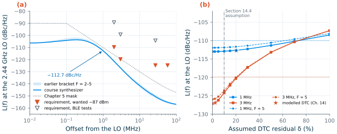
Chapter 14 first assumed that the digital-to-time converter (DTC) cancels the modulator’s timing error to a 10 % residual, and then modelled the DTC and its calibration; the budget above uses the model. Figure 19.4b shows how much rests on the cancellation, with a residual δ in place of the model. The 1 MHz point hardly cares: it holds −110 dBc/Hz up to a residual of 73 %. The 3 MHz point does: it meets −119.9 dBc/Hz only for residuals below 21 %, and without the DTC (100 %) both points fail, at −108.5 and −107.3 dBc/Hz. The calibrated DTC is worth δ = 2.4 % at 3 MHz, but 20 % at 1 MHz, where its own jitter, rounding and leftover INL add a white floor that a scaled residual does not have (the stars). The DTC is therefore load-bearing at 3 MHz, and its gain and INL must be calibrated; Section 19.5 shows the gain loop.
I/Q accuracy
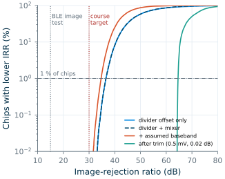
Chapter 5 allocated 0.2 dB of gain error and 2° of phase error to the whole I/Q path (33.6 dB of IRR). The largest designed contribution is the divide-by-two: Chapter 13 found its quadrature error to be 0.114° per millivolt of offset at its clock input, for 0.3 V of drive. The VCO delivers 0.335 V, so by Eq. (13.4) the sensitivity is 0.102°/mV. The offset comes from the threshold mismatch of the 6 µm × 0.13 µm clock pair, which by Pelgrom’s law [177], with the SG13G2 constant \(A_{VT}\) = 5.7 mV·µm extracted in The Art of Analog IC Design (Chapter 13), is
\[\sigma_{\theta} = \frac{d\theta}{dV_{os}}\,\frac{A_{VT}}{\sqrt{WL}} = 0.102\ ^\circ/\mathrm{mV}\times\frac{5.7\ \mathrm{mV\,\mu m}}{\sqrt{6 \times 0.13}\ \mathrm{\mu m}} = 0.102 \times 6.45\ \mathrm{mV} = 0.66^\circ. \tag{19.3}\]The mixer with its OTAs adds 0.005 dB and 0.044° (Chapter 10’s 1 % switch mismatch, taken as one standard deviation). The mismatch between the I and Q TIAs was not simulated, and the complex filter and the VGA were not designed; we assume 0.1 dB and 0.3° (one standard deviation) for them together. A Monte Carlo of 200 000 chips (Figure 19.5) gives a total phase error of 0.73° rms. Its 3σ value, 2.18°, exceeds the 2° allocation, and 0.60 % of the chips are beyond 2°; yet none of the 200 000 falls below 30 dB of IRR, because the designed gain error is far smaller than the 0.2 dB that Chapter 5 allowed. The median IRR is 42.9 dB and 99 % of the chips reach 34.7 dB. The behavioural runs below use that 1 % chip: 0.14 dB and −1.92°.
The behavioural receiver with the designed numbers
Chapter 5 checked its budget with a complex-envelope receiver: random GFSK data, real filters, a discriminator, bit errors counted. tools/figs/_ch19_rx.py imports its pieces and adds what Chapter 5 left out, all referred to the antenna:
- Noise for the designed NF, 4.62 dB, in absolute power: the wanted signal is specified in dBm.
- Nonlinearity: a third-order, saturating model of the front end (band filter, LNA and mixer, IIP3 = −7.1 dBm) on the complex envelope, and one of the baseband (IIP3 = −9.7 dBm at the antenna) on each real I and Q rail, where it can also mix interferers across zero frequency.
- The synthesizer’s phase noise, synthesized from the L(f) of Figure 19.4a (simulated VCO, modelled DTC), not a mask.
- The I/Q errors of the 1 % chip, the assumed band filter (a third-order 0.5 dB Chebyshev, 2400–2483.5 MHz) acting on each interferer at its absolute frequency, a carrier frequency offset of up to ±150 kHz removed by a digital estimate, and a 6-bit ADC on each rail with an ideal AGC that puts the rms 12 dB below full scale.
With Chapter 5’s inputs the new model reproduces Table 5.4’s tolerances within 1.1 dB, the resolution of a search in 2 and 3 dB steps, which checks the reimplementation.
Sensitivity and the carrier offset. Figure 19.6a shows the bit-error rate against the wanted power. With Table 5.3’s complex filter (4th-order Butterworth, 1 MHz noise bandwidth, cut-off 487 kHz) and no carrier offset, the BER reaches 10−3 at −96.9 dBm, within 0.2 dB of Eq. (4.12). But BLE allows a transmitter’s carrier to be 150 kHz off [184], and then the same receiver needs −91.7 dBm: the 1 MHz filter cuts into the shifted GFSK spectrum (99 % of its power within 1031 kHz), and the inter-symbol interference costs 5.2 dB even though the offset itself is removed digitally. Widening the filter to a 1.4 MHz noise bandwidth (cut-off 682 kHz) admits 1.5 dB more noise but recovers the shape: −97.2 dBm without offset, −96.3 and −96.2 dBm at +150 and −150 kHz. That is the filter this chapter recommends, and the one assumed from here on. Estimating the offset from each packet’s 8-bit preamble alone, instead of tracking it over many packets, costs another 0.7 dB (−96.5 dBm).
The ADC needs few bits: 6 bits at 12 dB of back-off lose nothing measurable (−97.2 against −97.0 dBm without an ADC, within the statistical scatter), 4 bits lose 1.4 dB. A limiting receiver with 1 or 2 bits needs a different back-off and is not modelled here.
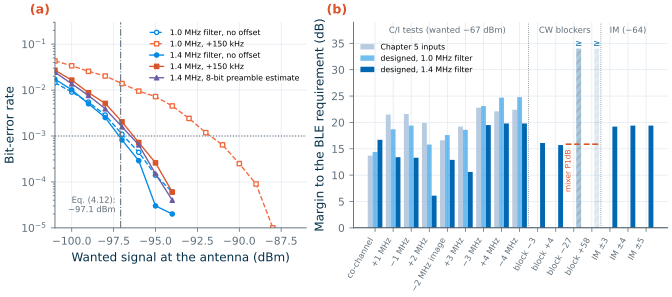
Interference, blocking and intermodulation. With Chapter 5’s inputs the model passes everything, as Table 5.4 did. With the designed numbers and the 1.0 MHz filter, every interference test passes by at least 14.4 dB (Table 19.3, Figure 19.6b). The 1.4 MHz filter that the carrier offset demands pays for its width in selectivity: it attenuates the channel 2 MHz away by 39.0 dB instead of 50.8 dB, and the +2 MHz margin falls from 15.8 to 6.1 dB, the smallest of all; the ±1 MHz and image margins shrink to about 13 dB. Every test still passes. The image margin, 12.9 dB, is no longer simply the IRR less 15 dB (Chapter 5): the wider filter lets more of the image channel itself through. Neither filter is the obvious optimum, and a design between them, or a sharper filter of higher order, is the next iteration.
BLE’s blocking test (Core Specification, Vol 6, Part A, §4.3) places the wanted signal at 2426 MHz [184]. We also run the edge channels, 2402 and 2480 MHz, with a CW interferer just outside the band at 2399 and 2484 MHz: §4.2 counts any interferer outside 2400–2483.5 MHz as out-of-band blocking, so the same −35 dBm applies. These blockers, 3 and 4 MHz from the wanted channel, are tolerated up to −18.9 and −19.3 dBm, 16.1 and 15.7 dB above the requirement; at those levels the blocker’s reciprocal mixing puts about −86 and −90 dBm into the channel, and the baseband rails, which clip at −15.7 dBm referred to the antenna, are within 3–4 dB of clipping. With the synthesizer’s lower noise beyond 2 MHz, the baseband’s compression now shares this limit with reciprocal mixing.
Far from the channel, 27 and 58 MHz away, the model never failed up to −1 dBm; but its saturation keeps the phase of the signal, as a limiter does, and a compressed transistor stage does not, so the honest limit there is the mixer’s 1 dB compression point of Section 19.2: the OTA’s −3.5 dBm at the mixer’s input, −19.1 dBm at the antenna, 15.9 dB above the requirement. Two blockers at once compress it sooner: Chapter 10’s two tones of −4 dBm each (−19.6 dBm at the antenna) cost 4.7 dB of gain.
In BLE’s intermodulation test the two −50 dBm interferers are tolerated up to −30.6 to −30.8 dBm for every n = ±3, ±4 and ±5 (BLE asks for only one of n = 3, 4, 5 to pass, so testing all of them is stricter), 19.2–19.4 dB above the requirement and about 2.5 dB better than Eq. (5.16) predicts with the cascaded IIP3 (−33.1 dBm), because the third-order product of a CW and a GFSK interferer is GFSK-like and the discriminator tolerates it at a lower C/I than noise, the pitfall of Chapter 5 again.
Table 19.3. BLE receiver tests against the behavioural course receiver. C/I tests: the C/I at which the BER reaches 0.1 % (wanted −67 dBm, GFSK interferer; offsets from the wanted channel, LO 1 MHz below it). Blocking: the CW blocker power at 0.1 % BER (wanted −67 dBm; BLE's §4.3 test uses 2426 MHz, the edge-channel cases follow §4.2). Intermodulation: the power of each of the two interferers, CW at f0 + n MHz and GFSK at f0 + 2n MHz (wanted −64 dBm). Margin in dB.
| Test | Requirement | Chapter 5 inputs | Designed, 1.0 MHz filter | Designed, 1.4 MHz filter |
|---|---|---|---|---|
| C/I, co-channel | 21 dB | 7.3 (13.7) | 6.6 (14.4) | 4.3 (16.7) |
| C/I, +1 MHz | 15 dB | −6.5 (21.5) | −3.7 (18.7) | 1.6 (13.4) |
| C/I, −1 MHz | 15 dB | −6.6 (21.6) | −4.4 (19.4) | 1.7 (13.3) |
| C/I, +2 MHz | −17 dB | −36.9 (19.9) | −32.8 (15.8) | −23.2 (6.2) |
| C/I, −2 MHz (image) | −9 dB | −25.6 (16.6) | −26.6 (17.6) | −21.9 (12.9) |
| C/I, +3 MHz | −27 dB | −46.2 (19.2) | −45.6 (18.6) | −37.6 (10.6) |
| C/I, −3 MHz (image − 1 MHz) | −15 dB | −37.8 (22.8) | −38.1 (23.1) | −34.5 (19.5) |
| C/I, +4 MHz | −27 dB | −49.1 (22.1) | −51.7 (24.7) | −46.8 (19.8) |
| C/I, −4 MHz | −27 dB | −49.4 (22.4) | −51.8 (24.8) | −46.8 (19.8) |
| Blocking, CW 2399 MHz, wanted 2402 MHz (edge channel; out of band by §4.2) | −35 dBm | −18.9 dBm (16.1) | ||
| Blocking, CW 2484 MHz, wanted 2480 MHz (edge channel; out of band by §4.2) | −35 dBm | −19.3 dBm (15.7) | ||
| Blocking, CW 2399 and 2484 MHz, wanted 2426 MHz (the §4.3 test) | −35 dBm | no failure up to −1 dBm in the model; mixer P1dB (single tone) −19.1 dBm (15.9) | ||
| Intermodulation, n = ±3, ±4, ±5 (BLE requires one of n = 3, 4, 5) | −50 dBm | −30.6 to −30.8 dBm (19.2–19.4) |
19.3 The transmit chain
The transmitter is the synthesizer, a second divide-by-two, a driver and the PA (Figure 19.1). GFSK is applied at two points, the fractional divider and the VCO’s tuning input (Chapter 14), the PA runs in compression, and its output network is the Q = 40 off-chip version of Chapter 16. Table 19.4 collects the results.
Output power and efficiency. The PA, with Chapter 16’s harmonic traps, delivers +10 dBm at 31.0 % PAE (33.7 % collector efficiency) from 14.9 mA at 2.0 V, 29.8 mW, with −2.2 dBm of drive. It saturates at +10.4 dBm, so it has 0.4 dB of headroom. That headroom is the problem of the whole chain. If, as in Figure 19.1, the transmitter shares the antenna with the receiver through the T/R switch and the band filter, Table 5.3’s 2 dB of loss applies to it too, and the antenna receives +8.0 dBm; delivering +10 dBm there would need +12.0 dBm from a PA that saturates 1.6 dB lower. The 0.60 mW of drive must also come from somewhere: the divide-by-two’s 1 kΩ CML output cannot deliver it into the PA’s 50 Ω input, so a driver stage, not designed in the course, sits in between. Counting the PA, VCO, transmit divider and prescaler, 32.8 mW, the transmitter turns 30.5 % of its DC power into +10 dBm, before the driver and the digital circuits.
Harmonics and spurs. Regulations measure emissions at the antenna. In Europe the limit from 1 to 12.75 GHz is −30 dBm [189]. In the United States both harmonics fall in restricted bands (4.5–5.15 and 7.25–7.75 GHz) [190], where the limit is a field of 500 µV/m at 3 m, an equivalent isotropically radiated power of −41.2 dBm. Chapter 16’s harmonic traps bring the second harmonic down to −65.0 dBm and the third to −61.2 dBm at the antenna, 35.0 and 31.2 dB inside ETSI’s limit and 23.8 and 20.0 dB inside the FCC’s (Figure 19.7b). Without traps the two were −52.6 and −21.8 dBm, and the third failed both limits; a 3f0 trap alone fixed the third but raised the second to 0.5 dB above the FCC limit, which the 2f0 trap at the output then removed at no cost in PAE. No extra filter is needed; one with 0.3 dB of loss would lower the PAE to 28.9 %. The synthesizer’s spurs are harmless here: the fractional spur at 2 MHz (Chapter 14’s worst case, 4 % charge-pump mismatch) is −57.0 dBm and the reference spur −102 dBm.
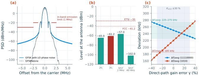
In-band emission. The LO’s phase noise spreads the carrier into the neighbouring channels. Through the designed synthesizer, the 1 MHz band at ±2 MHz receives up to −49.3 dBm and the bands at ±3 MHz −56.5 dBm (Figure 19.7a), 29.3 and 26.5 dB inside BLE’s −20 and −30 dBm limits [184]. At 2 MHz the GFSK spectrum itself (−55.7 dBm) and the phase noise (−50.8 dBm) contribute together; from 3 MHz on the phase noise alone sets the level.
Modulation accuracy. BLE specifies the transmitted deviation rather than an EVM. The Core Specification asks for a modulation index of 0.45–0.55, a minimum deviation of 185 kHz, and a deviation for 1010 patterns of at least 80 % of that for 00001111 patterns [184]; the RF test specification measures these as Δf1avg (over 11110000 patterns, 225–275 kHz), Δf2max (above 185 kHz) and Δf2avg/Δf1avg (at least 0.8), the names used here. The phase noise hardly matters: 0.41° rms and 1.60 kHz of rms frequency error against a 250 kHz deviation. The two-point modulator does. With matched paths the model gives Δf1avg = 250.0 kHz and Δf2avg = 219.8 kHz, a ratio of 0.879, set by GFSK’s own inter-symbol interference. Through the divider alone, without the VCO path, the 400 kHz loop passes the 500 kHz pattern so poorly that Δf2avg falls to 76.6 kHz. With the VCO path’s gain off by γ (Eq. (14.7)), Figure 19.7c shows Δf1avg barely moving and Δf2avg following γ almost linearly: the ratio drops below 0.8 for γ < −10 %, and Δf2 below 185 kHz near −25 %. The test tolerates a VCO path that is too strong far better than one that is too weak, but KVCO’s spread after band calibration, −21 % to +27 % around its design value (Chapter 11), covers both: the gain must be calibrated (Section 19.5).
Table 19.4. The course transmitter (2.44 GHz, tt, 27 °C; PA with the Q = 40 off-chip network, VPA = 2.0 V).
| Item | Requirement | Course transmitter | Margin |
|---|---|---|---|
| Output power at the PA | +10 dBm | +10 dBm (saturates at +10.4 dBm) | 0.4 dB of headroom |
| Output power at the antenna, through 2 dB of filter and switch | — | +8.0 dBm | PA would need +12.0 dBm |
| PAE at +10 dBm | ≥ 30 % | 31.0 % (collector efficiency 33.7 %) | 1.0 point |
| DC power: PA, VCO, divide-by-two, prescaler | — | 29.8 + 0.77 + 2.01 + 0.18 = 32.8 mW | driver not designed |
| 2nd harmonic | ≤ −30 dBm (ETSI), ≤ −41.2 dBm (FCC) | −65.0 dBm | 35.0 dB, 23.8 dB |
| 3rd harmonic | ≤ −30 dBm (ETSI), ≤ −41.2 dBm (FCC) | −61.2 dBm | 31.2 dB, 20.0 dB |
| In-band emission at ±2 MHz, ≥ ±3 MHz | ≤ −20 dBm, ≤ −30 dBm | −49.3 dBm, −56.5 dBm | 29.3 dB, 26.5 dB |
| Δf1avg, Δf2avg/Δf1avg (matched two-point paths) | 225–275 kHz, ≥ 0.8 | 250.0 kHz, 0.879 | needs γ ≥ −10 % |
| LO phase error, 10 kHz–8 MHz | — | 0.41° rms |
19.4 Spurs, coupling and self-interference
A block simulated alone cannot see the others. Three couplings matter most in this radio.
The PA’s second harmonic and the VCO
Chapter 5 placed the VCO at twice the carrier so that the PA’s output would not pull it (Chapter 5, Worked example 5.3). The second harmonic of the PA does fall on the VCO. How much coupling can the radio take? Adler’s equation (5.15) [71, 82] gives the lock range in terms of the injected and the oscillating currents. If a fraction of the PA’s harmonic power reaches the tank, the currents scale as the square roots of the powers that each delivers to the tank’s parallel resistance:
Key equation · Lock range for an injected power
\[f_L = \frac{f_0}{2Q}\sqrt{\frac{P_{inj}}{P_{osc}}}, \qquad P_{osc} = \frac{V_{osc}^2}{2R_p}, \qquad P_{inj} = P_{2f_c} - \mathrm{isolation} \tag{19.4}\]Within ±fL of its free-running frequency the VCO locks to the injection; a coherent injection shifts its frequency by up to fL.
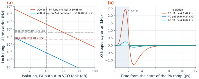
The course VCO has Q = 14.9, Rp = 906 Ω and 0.784 V of differential amplitude: Posc = −4.7 dBm and f0/2Q = 163.8 MHz. Its injection is the PA’s second harmonic, −65.0 dBm at the output with Chapter 16’s harmonic traps. With 40 dB of isolation between the PA’s output and the tank (Chapter 5’s “easily reached” coupling, our assumption), Eq. (19.4) gives fL = 1.58 kHz at the VCO. Had the VCO run at the carrier, it would receive the +10 dBm fundamental, 75.0 dB more, and fL would be 4.45 MHz, ten times the loop bandwidth (Figure 19.8a). BLE’s 50 kHz drift limit [184] applies to the carrier, and the divide-by-two halves the course VCO’s frequency error on its way there (0.79 kHz at 40 dB). To stay below it, the VCO at the carrier would need 79 dB of isolation; at twice the carrier, 4.0 dB.
The harmonic is also coherent: it is derived from the VCO itself, through the dividers and the PA, so it injects at exactly the VCO’s frequency with a fixed phase. That shifts the VCO’s free-running frequency by at most fL, which the type-II loop removes. The risk is the moment the injection changes: when the PA ramps up before a packet, the harmonic grows and its phase moves with the PA’s AM-PM (−33.5° at +10 dBm). We model the worst case, a VCO-referred frequency step of fL that grows with the square of a 2 µs raised-cosine ramp, and run it through Chapter 12’s closed loop (Figure 19.8b). With 40 dB of isolation the LO’s frequency moves by at most 0.24 kHz and settles in 4.1 µs; with 20 dB, 2.42 kHz and 6.2 µs. Both are small against BLE’s ±50 kHz drift and its 400 Hz/µs drift-rate limit once the packet starts [184]. The harmonic traps matter here too: with the 3f0 trap alone, whose second harmonic was 24 dB higher, the 20 dB case reached 39.7 kHz.
Common pitfall · Taking the isolation at the wrong node
The PA’s 2f0 traps keep the second harmonic off the output pin, −75.0 dBc, but inside the PA the class-AB collector current has a second harmonic only about 15 dB below the fundamental (Chapter 16’s conduction-angle analysis gives −15.3 dBc at 240°), and it circulates through the trap, the bond wires and the ground. That loop, not the antenna port, is what couples magnetically to the VCO’s spiral. The 40 dB in this section is an assumption about the whole path; the number that decides it comes from an electromagnetic simulation of the layout, the job of Chapter 18.
Reference and fractional spurs
Chapter 12’s estimate, −112 dBc for 1 nA of leakage and 4 % pump mismatch, is 52.7 dB inside the course requirement of −59.3 dBc, so coupling will set the real spur, as it did in the taped-out SG13G2 PLL (−40.2 dBc reported [106]). Turning Eq. (12.12) around gives the budget for coupling. A ripple of amplitude \(V_r\) at fref on the tuning line makes a spur \(S\) (dBc at the VCO, 6 dB above the LO) if
\[V_r = \frac{2f_{ref}}{K_{VCO}}\,10^{S/20}. \tag{19.5}\]For the course requirement this is 1.32 mV at 40 MHz with KVCO = 131 MHz/V, 1.04 mV at 167 MHz/V, the top of the calibrated range; for BLE’s emission limit alone, 12.2 mV. A millivolt of 40 MHz on a high-impedance node that runs past the reference buffer and the divider is easy to collect, which is why the third pole of Chapter 12 and a guarded, short tuning line matter. The fractional spur at 2 MHz, −67.0 dBc in Chapter 14’s worst case, needs to stay below −49.7 dBc for a −50 dBm interferer 2 MHz away from a wanted signal at −87 dBm: 17.3 dB to spare.
LO leakage and DC offset
With matched switches the four 25 % LO phases cancel at the mixer’s RF node (Chapter 10). Take the gate-drain capacitance as 30 % of the 79.6 fF switch gate and a 1 % mismatch between phases (both assumptions): a residue of 0.24 fF, driven by the 0.54 V fundamental of each 25 % pulse, injects 1.98 µA at 2.44 GHz. Into the 18 Ω of the RF node (the LNA’s 50 Ω output in parallel with the mixer’s 28 Ω input) that is 35.8 µV, −78.9 dBm at the mixer. Through the LNA’s reverse isolation (S12 = −38.1 dB) and the filter, −119.0 dBm reaches the antenna, below the thermal noise in 1 MHz. The same leak, reflected and self-mixed, makes a DC offset of microvolts.
The DC offset that does matter comes from the TIAs’ OTAs (σ = 0.11 mV each, Chapter 10), whose offset Chapter 10’s noise gain of 1.71 multiplies. In a low-IF receiver it sits 1 MHz below the channel, and the complex filter attenuates zero frequency by 25.3 dB with the 1 MHz filter and 13.7 dB with the recommended 1.4 MHz filter, before the ADC. A DC servo or a high-pass corner of a few tens of kilohertz, which Chapter 5 found costs nothing at a 1 MHz IF, keeps the remainder from eating the ADC’s range.
19.5 Calibration and digital assistance
Several of the margins above exist only after calibration. Table 19.5 lists them; Figure 19.9 shows two.
Table 19.5. Calibrations of the course radio: what, why and how well (numbers from this chapter's models).
| What | Why | How | Result |
|---|---|---|---|
| VCO band | 16 bands of 32.6 MHz; process and temperature move the tank | count LO cycles for 10 reference periods (0.25 µs), binary search over 4 bits (Section 11.8 simulates it) | about 5 µs per channel; bands overlap 3.5 times |
| DTC gain | residual must stay below 21 % (Figure 19.4b) | sign-sign LMS on the bang-bang phase-detector output | 30 % → < 10 % in 12.9 µs, < 2 % in 18 µs (μ = 4 × 10⁻⁴) |
| Two-point gain | Δf2avg/Δf1avg ≥ 0.8 needs γ ≥ −10 %; KVCO spreads −21 % to +27 % after band calibration | measure KVCO: step the fraction, read the tuning voltage (or LMS on the phase error) | to a few percent |
| I/Q phase and gain | IRR ≥ 30 dB with margin | factory: test tone, trim the divider’s clock-input offset (0.051° per 0.5 mV step) and the VGA gain (0.02 dB) | 1 % point of IRR from 34.7 to 64.6 dB |
| DC offset | TIA op-amp offsets eat ADC range | DC servo or high-pass of tens of kHz | no BER cost at 1 MHz IF (Chapter 5) |
| Carrier offset | up to ±150 kHz at the transmitter (BLE’s limit), plus the receiver’s own LO error | estimate on the preamble, track over packets | 0.6 dB from the preamble alone |
| PA power | optional in BLE (LE Power Control, steps of at most 8 dB); saves energy on short links | lower the drive, or scale the PA supply | at 0 dBm: 10.7 % or 20.4 % collector efficiency |
DTC gain. The DTC delays each divider edge by its predicted timing error, a swing of 1.6 ns for the MASH 1-1-1. If its gain is off by δ, the phase detector sees δ times the error, correlated with the prediction. A bang-bang detector’s sign, multiplied by the sign of the prediction, therefore points the way to the right gain, and a sign-sign LMS loop [176] steps the gain by μ each reference cycle. We ran it on the bit-exact MASH 1-1-1 sequence of the 2442 MHz channel from Chapter 14, with 0.5 ps of random timing noise standing for the loop’s own phase noise and a starting error of 30 % (Figure 19.9a). With μ = 4 × 10⁻⁴ the error falls below 10 % in 12.9 µs and below 2 % in 18 µs, and wanders by 0.08 % rms afterwards; with μ = 10−4, 51.4 and 71.9 µs, 0.04 %. At δ = 2 % the 3 MHz phase noise improves from −124.3 dBc/Hz (the 10 % residual) to −127.0 dBc/Hz. The model ignores the DTC’s nonlinearity. Chapter 14 models it: a 10 ps bow and 2 ps segment steps leave a −105.9 dBc/Hz floor and a −67.5 dBc spur at 2 MHz even with the gain calibrated, so the INL needs its own calibration; with a 16-segment pre-distortion [176] the synthesizer meets both specifications, and the DTC is worth an effective 2.4 % residual at 3 MHz. That calibrated DTC is the one this chapter’s synthesizer uses (Section 19.2).
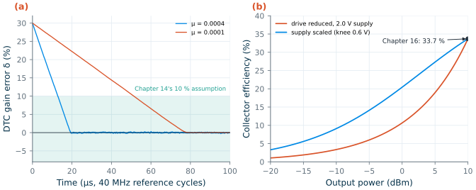
PA power control. BLE does not require it. The Core Specification bounds only the output power at the maximum setting, measured at the antenna connector, which sets the power class [184]: Class 1.5 covers more than +4 up to +10 dBm, so the course PA’s +10 dBm is the top of that class, and the +8.0 dBm that reaches the antenna through the shared filter and switch lies inside it. Power control is optional, in steps of at most 8 dB under LE Power Control. Still, a link close to its peer should not spend +10 dBm. Lowering the drive keeps the 2.0 V supply and the quiescent current, and a class-B-like stage loses efficiency in proportion to its output amplitude: 33.7 % at +10 dBm becomes 10.7 % at 0 dBm and 3.4 % at −10 dBm (Figure 19.9b). Lowering the supply instead, with a DC-DC converter, keeps the stage near saturation; only the 0.6 V knee of the cascode, now a larger part of the supply, costs efficiency: 20.4 % at 0 dBm (1.04 V) and 9.1 % at −10 dBm (0.74 V). This is average power tracking, which the smartphone of Section 19.6 uses for its cellular PAs.
What this means for your design
Calibration is part of the architecture, not a repair. Each loop above needs a measurement path (a counter, the phase detector’s sign, a test tone, the ADC), a place to act (a capacitor bank, a DTC gain register, an offset DAC, a supply), and time in the radio’s schedule. Plan them with the blocks: the divider’s 0.1° per millivolt that causes the I/Q error is also the knob that trims it.
19.6 Case study: a smartphone RF front-end
The course radio is a single-standard, single-antenna radio. A smartphone carries a dozen of them. Pretl’s course notes [1] end with a walk through the published schematics of the Fairphone (Gen. 6), and the comparison is instructive. The summary below paraphrases that appendix; the part numbers and functions come from it, and through it from the schematic labels.
Architecture. The phone covers 2G to 5G below 7.125 GHz, Wi-Fi 6E with 2 × 2 MIMO, Bluetooth, satellite navigation (GNSS) in two bands and NFC. The application processor and the modem share one SoC; one RF transceiver IC handles all cellular bands and GNSS and exchanges I/Q samples with the modem over a fast serial link; a separate combo chip handles Wi-Fi and Bluetooth with its PAs on chip. The cellular transceiver has four receive groups, for 4 × 4 downlink MIMO, two transmit chains, a feedback receiver input and two GNSS inputs, and no IF filters: it is a direct-conversion transceiver, the zero-IF architecture of Chapter 5. Its LOs cover more than six to one, from 617 MHz to 3.8 GHz, with divide-by-two stages that also make the quadrature, as in the course radio; by Pretl’s estimate that takes three VCOs per synthesizer.
Front end. Everything the course radio leaves to “band filter + T/R switch” is a module there. Eleven antenna feeds serve MIMO, concurrent radios and sounding; diplexers and triplexers share antennas between bands (one antenna carries a cellular downlink band, GNSS L1 and 2.4 GHz Wi-Fi); antenna tuners match the low-band antennas; most frequency-division bands need their own acoustic duplexer, whose transmit-to-receive gap of 10–20 MHz asks for a quality factor near 100. The LNAs are separate modules ahead of the transceiver, because the losses in front of them (diplexer, switch, filter) would otherwise add directly to the NF. The multimode PA modules each have their own DC-DC converter for average power tracking, and a directional coupler feeds a sample of the output back to the transceiver for power control, I/Q and LO-leakage calibration and predistortion: the calibration paths of Section 19.5, made explicit. Dual uplink in two bands at once creates intermodulation products that land in the phone’s own receive bands; keeping them below the noise would need an IIP3 near +85 dBm, so the standard permits a defined loss of sensitivity instead.
The course radio in such a phone. Bluetooth shares the 2.4 GHz ports and antennas with Wi-Fi. Suppose the course receiver sat behind the same kind of front end (Figure 19.10): a diplexer, an antenna switch and a filter, which we assume lose 0.4, 0.7 and 1.5 dB (2.6 dB in total, instead of Table 5.3’s 2 dB). The NF rises from 4.62 to 5.22 dB and the sensitivity to −96.5 dBm, still 6.5 dB inside the course’s −90 dBm.
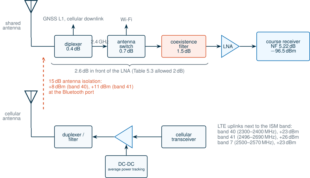
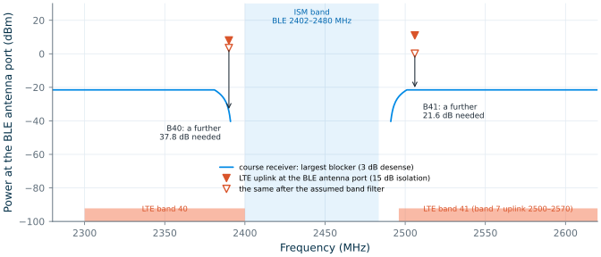
The real issue is the phone’s own transmitters. LTE band 40 (2300–2400 MHz) ends at the ISM band’s lower edge, and band 41 (2496–2690 MHz) and band 7’s uplink (2500–2570 MHz) start 12.5 MHz above its upper edge; the Fairphone supports all three, band 41 at the higher power class. Assume 15 dB of isolation between the cellular and Bluetooth antennas. A band-40 uplink at +23 dBm, centred 12 MHz below the 2402 MHz channel, then arrives at the Bluetooth port at +8 dBm; band 41 at +26 dBm, 26 MHz above 2480 MHz, at +11 dBm. How much can the course receiver take? Reciprocal mixing sets the limit: a blocker that spreads, through the LO’s phase noise, as much power into the channel as the thermal noise desensitizes the receiver by 3 dB:
\[P_{B,max} = \left(-174 + \mathrm{NF} + 10\log_{10}B\right) - \overline{\mathcal{L}} - 10\log_{10}B, \qquad R \ge P_{TX} - I_{ant} - P_{B,max}, \tag{19.6}\]where \(\overline{\mathcal{L}}\) is the LO’s phase noise averaged over the offsets the blocker occupies (a 20 MHz LTE channel here), \(R\) the rejection a filter must provide and \(I_{ant}\) the antenna isolation. For band 40, 2–22 MHz from the 2402 MHz channel, the designed synthesizer averages −134.5 dBc/Hz and PB,max = −34.3 dBm; for band 41, 16–36 MHz from 2480 MHz, it averages −149.5 dBc/Hz, so reciprocal mixing would allow −19.2 dBm. Further out, compression comes first. The OTA mixer compresses by 1 dB at −3.5 dBm at its input (Section 19.2), which is −18.5 dBm at the phone’s antenna port, 2.4 dB before the cubic estimate from the front end’s IIP3 (−16.1 dBm). A blocker 3 dB below the compression point costs the wanted signal about 1 dB of gain (Section 4.7), so −21.5 dBm is the limit for bands 41 and 7. Figure 19.11 shows the result: band 40 needs 42.3 dB of rejection at 2390 MHz, band 41 32.5 dB at 2506 MHz and band 7 29.5 dB at 2510 MHz, while the assumed three-pole band filter provides 4.5, 10.9 and 12.7 dB. A coexistence filter with steep acoustic skirts must find the remaining 37.8, 21.6 and 16.8 dB, within about 10 MHz of the band edge. No receiver design removes the other half of the problem: the LTE transmitter’s own noise inside the ISM band, which must be below −122.8 dBc/MHz (relative to +23 dBm) to stay 6 dB under the course receiver’s noise floor. That falls to the cellular side’s filters, and, where they cannot reach it, to the two radios taking turns in time.
What this means for your design
In a phone, a receiver’s hardest numbers come from its neighbours, not from its own standard. BLE’s blocking test asks for −35 dBm; the phone’s band-40 transmitter delivers +8 dBm. The course synthesizer’s far-out phase noise and the front end’s compression set the receiver’s half of the answer, and a filter, the antenna layout and the radios’ scheduling set the rest. Chapter 5’s budget would be written differently for such a product: start from the coexistence cases, and let BLE’s tests be the easy ones.
19.7 Where to go next
Lay it out and tape it out. The course has carried the design to schematics with EM-fitted passives; Chapter 18 shows the next steps, layout, design-rule checks and electromagnetic extraction, on the millimetre-wave PA’s matching networks and the pads, and the same steps apply to every block here. IHP runs open multi-project-wafer (MPW) shuttles for open-source designs in SG13G2 [191, 211]. The April 2025 run alone carried a 160 GHz LNA, 180 GHz PAs, a 5 GHz upconversion mixer, VCOs, a GPS-band LNA, RISC-V systems and Tiny Tapeout shuttles [211, 5]. Small dies with GSG pads for the LNA, the VCO with its divider, and the PA are realistic first chips; the full transceiver needs the calibration logic of Section 19.5 as well.
Measure. Each block’s measurement checks one assumption of this chapter. The LNA’s S-parameters, after the open–short de-embedding of Chapter 3, and its noise figure by the Y-factor method check Chapter 9 and the pad capacitance; the mixer’s conversion gain, noise figure and compression check Chapter 10’s simulation with the transistor-level OTA; a phase-noise measurement of the VCO and the closed loop checks Chapter 11’s simulated phase noise and Chapter 14’s DTC model; a load-pull of the PA checks Chapter 16’s network loss; and a bit-error-rate test with a BLE tester closes the loop on Figure 19.6.
Close the thin spots. The weakest numbers are known: the mixer’s OTA with real capacitors and resistors, a layout and its corners (Chapter 10 simulates it at the typical corner only, and its noise figure with behavioural switches), a transformer or a third-harmonic termination for the PA (Chapter 16), the corners of the mixer and the synthesizer, and a transistor-level complex filter, VGA and ADC from the sibling course, The Art of Analog IC Design [4]. Each would turn an assumption of this chapter into a simulation.
Try it · The transceiver script
Every number in this chapter comes from
tools/figs/ch19_transceiver.pyand its receiver modeltools/figs/_ch19_rx.py:python3 tools/figs/ch19_transceiver.pyredraws everything in about a minute from cached behavioural runs, andrx --resimreruns the receiver (about ten minutes). Three experiments: (1) InASSUME, lower the band filter and switch loss from 2 to 1 dB (filter_switch) and runcascade blocks: how much of the 1 dB reaches the sensitivity, and why more than half? (2) Inrx_part, change the 1.4 MHz filter (1.4e6) to 1.2 MHz and runrx --resim: how much of the +150 kHz sensitivity do you keep, and how much of the +2 MHz interference margin do you win back? (3) InASSUME, setramp_usto 0.5 and runcoupling: how large is the kick for 20 dB of isolation in Figure 19.8b, and does it still settle before a packet could start?
- Checked against Table 5.3, the receiver, synthesizer and off-chip PA (with Chapter 16’s harmonic traps) pass; only the on-chip PA fails, on output power and PAE, and the mixer’s gain and NF, now simulated with a transistor-level OTA in its TIAs (Chapter 10), sit just inside their targets, by 0.05 and 0.12 dB.
- The designed receive chain reaches NF 4.62 dB, IIP3 −11.6 dBm, an IIP2 of at least +25.9 dBm at the antenna and a sensitivity of −97.1 dBm; the band filter and switch carry 55 % of the noise, and the mixer’s NF could be 9.6 dB worse before the 8 dB specification is reached. The mixer’s OTA compresses first: 1 dB at −19.1 dBm at the antenna.
- In the behavioural receiver, Table 5.3’s 1 MHz channel filter loses 5.2 dB to BLE’s ±150 kHz carrier offset; a 1.4 MHz filter keeps the sensitivity at −96.2 dBm or better. With it every BLE test passes: interference by at least 6.1 dB (at +2 MHz), blocking by 15.7–16.1 dB (the far blockers by 15.9 dB, the mixer’s 1 dB compression point), intermodulation by 19 dB.
- The divider’s mismatch gives 0.73° rms of I/Q phase error, more than 2° at 3σ, yet 99 % of chips exceed 34.7 dB of IRR; the synthesizer, with Chapter 11’s simulated VCO and Chapter 14’s calibrated DTC, has 2.7 dB of margin at 1 MHz and 7.0 dB at 3 MHz; a cancellation residual above 21 % would fail 3 MHz, and a sign-sign LMS calibrates the DTC’s gain in under 20 µs.
- The transmitter delivers +10 dBm at 31.0 % PAE but only +8.0 dBm through the shared filter and switch; with Chapter 16’s harmonic traps both harmonics clear the ETSI and FCC limits by 20 dB or more. Its spectrum (−49.3 dBm at 2 MHz) and modulation (Δf2avg/Δf1avg = 0.879) pass once the two-point gain is calibrated to γ ≥ −10 %.
- Running the VCO at 2fc cuts PA pulling by 75.0 dB; reference spurs will be set by coupling (1.3 mV of 40 MHz ripple on the tuning line is enough to fail), and in a phone the LTE transmitters next to the ISM band need a coexistence filter of 17–38 dB beyond a simple band filter.
Further reading
- BRICD, Designing a Serial Link from Scratch, Part III · Transceiver Circuits: the transmitter and receiver circuits of a 5 Gb/s serial link in SG13G2, the wireline counterpart of this chapter’s radio.
- H. Pretl, Radio-Frequency Integrated Circuits [1]: course notes from JKU Linz whose last appendix walks through the RF front end of the Fairphone (Gen. 6), the source of Section 19.6.
- F.-W. Kuo et al. [174] and S. Binsfeld Ferreira et al. [175]: a complete Bluetooth Low Energy transceiver with a 2.75 mW receiver and a switchable on-chip TX/RX matching network, and the system design behind its receiver; a measure of how far the course radio’s receive chain, at least 24.9 mW before its baseband, is from the state of the art.
- B. Razavi, RF Microelectronics [6]: transceiver architectures, the link budget and its interactions, and injection pulling, at much greater depth.
- S. Pamarti, L. Jansson and I. Galton [149]: a 2.4 GHz fractional-N synthesizer with 1 Mb/s in-loop modulation, the alternative to the course’s two-point modulator.
- S. Levantino, G. Marzin and C. Samori [176]: adaptive calibration of the gain and the nonlinearity of a DTC in a fractional-N PLL.