Lab 4
The 2.4 GHz LNA
Run the course LNA of Chapter 9 as a testbench of your own: S-parameters and noise from ngspice, read and checked with scikit-rf, the noise circles that the four noise parameters draw, a two-tone test in Xyce, and the same again at the fast corner and 85 °C.
- Build the course LNA’s netlist from Chapter 9’s script and run its
spanalysis with noise and its two-tone harmonic balance yourself.- Read the results into a scikit-rf
Networkwith its noise parameters, and refer them to the 290 K of the noise-figure definition.- Measure the gain, the input match and its bandwidth, NF and NFmin, the stability factors and the IIP3, and compare each with Chapter 9.
- Draw the noise circles and say why the 50 Ω source is not the noise optimum.
- Repeat the checks in a process corner and explain what moves.
Contents
| Lab 4 at a glance | |
|---|---|
| Goal | The course LNA’s gain, match, noise, stability and linearity from your own runs, at the typical corner and at ff, 85 °C. |
| Chapters | Chapter 9 (Sections 9.4, 9.5 and 9.7, Tables 9.2–9.4, Worked example 9.1); Chapter 4 for NF and IIP3 |
| Time | 3 hours |
| Files | tools/labs/lab4/: lna_lab.py; it imports tools/figs/ch09_lna.py (the netlist) and tools/figs/ch04_noise_linearity.py (harmonic-balance post-processing) |
| Run time | ngspice sp under a second; Xyce two-tone about 4 s; lna_lab.py all about 10 s |
Hand calculation
The course LNA (Figure 9.5) has \(L_g\) = 13.98 nH off chip with Q = 40, \(L_s\) = 0.823 nH, M1 of 128 µm at 4.70 mA, and a pad with ESD diodes. Before you simulate:
- Input Q and match bandwidth. Eq. (9.10) gives the loaded Q of the input network, \(Q_L = \omega_0(L_g + L_s)/R_S\). Compute it at 2.44 GHz. For a series resonant input matched to \(R_S\), the reflection is \(\Gamma = jX/(2R_S + jX)\) with \(X \approx 2Q_LR_S\,\Delta f/f_0\), so \(\vert S_{11}\vert\) = −10 dB where \(X = 2R_S/3\). Show that the −10 dB bandwidth is \(2f_0/(3Q_L)\) and evaluate it.
- Noise figure. Add up Eq. (9.9) with the four terms of Worked example 9.1: \(R_{Lg}/R_S\) = 0.107, \(R_g/R_S\) = 0.0672, \(R_{Ls}/R_S\) = 0.0268 and the channel term 0.176. Give F and NF.
- The hot corner. Every term of \(F - 1\) is thermal noise, so to first order it scales with the absolute temperature (the reference source stays at 290 K). Starting from the simulated \(F - 1\) = 0.309 at 27 °C, predict the NF at 85 °C.
- Linearity at the corner. Section 9.5 found that OIP3 = IIP3 + G stays near +12.7 dBm because the drain swing sets it. If OIP3 did not move, what IIP3 would a gain of 17.36 dB give?
Steps
Work in tools/labs/lab4 of the course files. Inside the container, run the commands as shown; from your own computer, put ../common/iic.sh in front of each one (Lab 0 shows how). Every step writes its netlist into out/, runs the simulator there, and prints what it measured.
-
S-parameters and noise.
cd /foss/designs/rfic-design/tools/labs/lab4
python3 lna_lab.py sp                 # from your computer: ../common/iic.sh python3 lna_lab.py sp
The script builds the netlist with
lna_lines()of Chapter 9’s script, from the design values at its top, writes it asout/lna_tt27_sp.cir(tag = corner and temperature) and runsngspice -bon it. Open the netlist. You will find every part of Figure 9.5:Lgwith its series resistanceRlgfor Q = 40, the pad capacitance and the two ESD diodes, the DC blockXCin, the 1:16 bias mirror, M1 and M2 as 16 RF cells each (rfmode=1), the EM-fitted π models of \(L_s\) and \(L_d\), andXC1,XC2of the output match. Its.controlblock runs an operating point (out/lna_tt27_op.txt), anspanalysis from 1 to 4 GHz with noise, written withwrs2pasout/lna_tt27.s2pand withwrdataas the noise-parameter tableout/lna_tt27_noise.txt, and a secondspfrom 0.1 to 30 GHz for the stability check (out/lna_tt27_wide.s2p). -
Read the results with scikit-rf [30, 215].
lna_lab.pydoes this inload_sp()andanalyse_sp(); do it once by hand to see each piece. Startpython3in the lab folder:import skrf as rf, numpy as np lna = rf.Network("out/lna_tt27.s2p") lna["2.44GHz"].s_db # |S11| |S12| / |S21| |S22| in dB from lna_lab import load_sp net, wide, nf_ngspice, op = load_sp("tt27", 27) k = np.argmin(abs(net.f - 2.44e9)) net.nfmin_db[k], net.g_opt[k], net.rn[k] # the four noise parameters, at 290 K 10 * np.log10(net.nf(50.0))[k] # NF for a 50 ohm source, from the noise parameters wide.stability.min() # Rollett's K, 0.1-30 GHzload_sp()attaches the noise parameters withNetwork.set_noise_a(). ngspice refers its noise figures to the circuit temperature, 27 °C here, so the script first converts them to the 290 K of the definition, as Chapter 4 does: \(F_{290} = 1 + (F - 1)\,T/T_0\) for \(F\) and \(F_{min}\), and \(R_n\,T/T_0\). Comparenet.nf(50.0)with ngspice’s ownnfcolumn after the same conversion (nf_ngspiceabove): scikit-rf recomputes the noise figure from \(F_{min}\), \(R_n\) and \(\Gamma_{opt}\) alone, so agreement shows that the four parameters describe the two-port’s noise completely. -
The noise circles. For a source reflection \(\Gamma_s\) every noise figure above \(NF_{min}\) is reached on a circle around \(\Gamma_{opt}\) (Chapter 6, Eq. (6.11)).
net.nf_circle(nf)returns the circle for a noise figurenfin dB at every frequency; take the column of 2.44 GHz. The script draws four of them, including the one through the 50 Ω point, intoout/lab4_sp_tt27.png(Figure L4.1b). -
Two-tone test in Xyce.
python3 lna_lab.py iip3It writes
out/lna_tt27_2tone.cir, Chapter 9’s harmonic-balance netlist: the same LNA (lna_lines()without the ports) between a 50 Ω source with two tones at 2.440 and 2.441 GHz and a 50 Ω load,.hbwith five harmonics per tone, and.stepover nine powers from −40 to −20 dBm per tone. Xyce [195] runs with the PSP plugin, andrfmode=1works in Xyce (see the PDK note in Section 9.7). The script readsout/lna_tt27_2tone.cir.HB.FD.prn, refers the outputs to available powers and fits lines of slope 1 and 3 through the three lowest points, as the chapter does. It also prints the slopes it actually finds there and between −27.5 and −20 dBm. -
One corner. Rerun both steps with fast MOSFETs at 85 °C, the corner where Table 9.3 found the worst match and the lowest IIP3:
python3 lna_lab.py sp iip3 --corner ff --temp 85Only the
mos_ttword of the.libline and the temperature change; the passives stay typical and the reference current stays 312.5 µA, as in Chapter 9. -
Everything at once.
python3 lna_lab.py allruns steps 1, 4 and 5, stores the checkpoint numbers inlab_numbers.jsonand draws Figure L4.1 and Figure L4.2 intoout/.
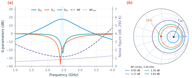
sp read with scikit-rf (tt, 27 °C; NF at 290 K). (a) S-parameters, NF for a 50 Ω source and NFmin; shaded: 2.400–2.4835 GHz. (b) Noise circles at 2.44 GHz from Network.nf_circle(): NFmin + 0.1, + 0.5 and + 1 dB, and the circle through the 50 Ω source.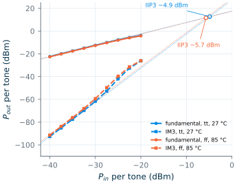
Checkpoint
Table L4.1. Lab 4 results (SG13G2, tt, 27 °C unless stated; band 2.40–2.49 GHz on the 10 MHz grid; NF at 290 K). Tolerance: ±1 in the last digit shown, except where stated.
| Quantity | Lab 4 | Chapter 9 |
|---|---|---|
| Hand calculation: \(Q_L\), −10 dB bandwidth \(2f_0/3Q_L\) (±5 %) | 4.54, 358 MHz | 4.54 |
| Hand calculation: NF from Eq. (9.9); NF at 85 °C from \(F - 1\) (±0.02 dB) | 1.39 dB; 1.36 dB | 1.39 dB |
| Hand calculation: IIP3 at ff, 85 °C if OIP3 stayed at +12.7 dBm | −4.7 dBm | |
| Supply current, power; VG, VX | 4.70 mA, 5.64 mW; 0.664, 0.498 V | 4.70 mA, 5.64 mW; 0.664, 0.498 V |
| S21 at 2.44 GHz; band minimum | 17.61 dB; 17.43 dB | 17.61 dB; 17.43 dB (Tables 9.2, 9.4) |
| S11 at 2.44 GHz; band maximum | −20.97 dB; −15.39 dB | −20.97 dB; −15.39 dB |
| −10 dB return-loss band | 2.230–2.609 GHz, 379 MHz | 2.23–2.61 GHz, 379 MHz |
| S22 at 2.44 GHz, band maximum; S12 | −19.48, −12.71 dB; −38.12 dB | −19.48, −12.71 dB; −38.12 dB |
| NF at 2.44 GHz (scikit-rf, 50 Ω); band maximum | 1.17 dB; 1.18 dB | 1.17 dB; 1.18 dB |
NF from ngspice’s nf column, converted to 290 K |
1.17 dB | |
| NFmin, \(R_n\), \(\Gamma_{opt}\) at 2.44 GHz | 0.83 dB, 12.5 Ω, 0.459∠−2.4° | NFmin 0.83 dB |
| K minimum (0.1–30 GHz), at; μ minimum above 1 GHz | 5.23 at 2.51 GHz; 1.02 | 5.23 at 2.51 GHz; 1.02 |
| Two-tone: IIP3, OIP3 (±0.1 dB) | −4.9 dBm, +12.7 dBm | −4.9 dBm, +12.7 dBm |
| Two-tone: gain of the slope-1 fit; slopes at −40 to −35 dBm | 17.61 dB; 1.00 and 3.04 | 17.62 dB (one tone at −40 dBm); 1.00 and 3.04 |
| IM3 slope between −27.5 and −20 dBm (±0.05) | 3.55 | 3.57 (Section 9.7) |
| ff, 85 °C: current; S21 band | 5.01 mA; 17.12–17.37 dB | 5.01 mA; 17.12–17.37 dB (Table 9.3) |
| ff, 85 °C: NF band maximum; S11 band maximum | 1.38 dB; −13.7 dB | 1.38 dB; −13.7 dB |
| ff, 85 °C: IIP3, OIP3 (±0.1 dB); NFmin; K minimum | −5.7 dBm, +11.7 dBm; 1.00 dB; 4.49 | −5.7 dBm |
Every row that Chapter 9 also reports agrees with it, the IIP3 and the slopes to the digits shown. Only the steep IM3 slope between −27.5 and −20 dBm, where the fifth-order products take over (Section 9.7), comes out 0.02 below the chapter’s; the chapter’s sweep continued to −5 dBm, and that last digit of a difference quotient is within the harmonic balance’s convergence tolerance. The match bandwidth of the hand calculation is 6 % narrower than the simulation: \(Q_L\) counts only \(L_g + L_s\), while the pad capacitance and \(C_{gd}\) change how fast the input reactance moves with frequency. At ff, 85 °C the hand calculation’s −4.7 dBm misses by 1 dB: the output intercept did not stay constant (Questions).
Questions
- \(\Gamma_{opt}\) is 0.459 at almost zero angle, so the optimum source is about 135 Ω, real. Why does the inductively degenerated stage not put its noise optimum at 50 Ω, and which element of the design would you change to move it there? What would that do to the input match?
- Hand calculation 3 predicted 1.36 dB at 85 °C from the temperature alone, and the simulation gives 1.37 dB at 2.44 GHz at ff. Which effects of the fast corner push the noise figure up and which push it down?
- At ff, 85 °C the gain fell by 0.25 dB but the IIP3 by 0.8 dB, so OIP3 dropped by about 1 dB. Look at \(V_X\) in the printout (0.498 V at tt, 0.564 V at ff, 85 °C) and explain with the drain-swing argument of Section 9.5.
- Rollett’s K is above 4 everywhere, yet μ approaches 1.02 above 1 GHz. Which S-parameter makes μ so close to one, and why does that not mean the amplifier is close to oscillating?
Extension
Replace the Q = 40 chip inductor by an on-chip spiral: set qlg=11.3 in LNA at the top of lna_lab.py (the Q of Chapter 7’s largest spiral) and rerun python3 lna_lab.py sp. Compare NF and NFmin with Figure 9.7: which of the two moves, and why does the other stay put? Then try the design trade of Table 9.2: change ld to 3.0 (nH) without rematching and run sp iip3. How much of the table’s 0.9 dB gain increase and 1.4 dB IIP3 loss do you get, and what does the mismatch at the output cost you?