Chapter 10
Mixers
The mixer moves the wanted channel from 2.4 GHz to the 1 MHz IF where the course receiver filters and demodulates it. It does so by switching, not by multiplying, and the way it switches decides its gain, its noise and how well it tolerates strong interferers. This chapter builds the arithmetic of switching mixers, compares passive and active mixers, and designs the course I/Q mixer in SG13G2: a 25 % duty-cycle current-mode passive mixer with transimpedance amplifiers.
- Explain mixing by nonlinearity and by time variance, and compute the conversion gain of a switching mixer from the Fourier series of its LO.
- Distinguish SSB and DSB noise figures, and explain why the low-IF receiver’s I/Q mixer is specified by its SSB noise figure.
- Analyse the current-mode passive mixer with a TIA: 50 % against 25 % LO, switch sizing against LO power, and the noise of each part.
- Compare the passive mixer with the Gilbert cell in gain, noise, linearity and power.
- Design and simulate the course I/Q mixer, including its noise figure by transient noise and by periodic small-signal analysis and the transistor-level op-amp of its TIAs, and check it against the Chapter 5 budget.
Contents
- 10.1 Mixing: nonlinearity and time variance
- 10.2 Conversion gain and noise figure of a mixer
- 10.3 Passive mixers
- 10.4 Active mixers and the Gilbert cell
- 10.5 Linearity and port-to-port isolation
- 10.6 N-path filters and mixer-first receivers
- 10.7 Quadrature LO generation
- 10.8 The course I/Q mixer
- Further reading
10.1 Mixing: nonlinearity and time variance
A linear time-invariant circuit cannot create a new frequency. A mixer must therefore be either nonlinear or time-variant. The textbook picture, Eq. (5.8), is a multiplier: \(\cos\omega_{RF}t\cdot\cos\omega_{LO}t\) contains \(\omega_{RF} \pm \omega_{LO}\). A nonlinear mixer gets the product from the square term of a device characteristic: apply \(v_{RF} + v_{LO}\) to a square-law device and the cross term \(2\alpha_2v_{RF}v_{LO}\) is the wanted product, together with every other product of the power series. Such mixers survive at millimetre waves, where nothing switches well, but their gain depends on the LO amplitude and their output is full of spurious terms.
Every mixer in a CMOS receiver below a few tens of gigahertz is instead a time-variant circuit: a switch, opened and closed by the LO, in the path of the RF signal. For the RF signal, which is small, the switch is a linear element whose conductance changes periodically, a linear periodically time-varying (LPTV) circuit [6]. Its output is the RF signal multiplied by a periodic waveform \(m(t)\), the switch’s mixing function, whose Fourier series
\[m(t) = \sum_{n} c_n e^{jn\omega_{LO}t} \tag{10.1}\]sets everything that follows. The fundamental \(c_1\) converts the wanted channel to the IF; the harmonics \(c_3, c_5, \dots\) convert signals and noise near \(3f_{LO}, 5f_{LO}, \dots\) to the same IF. Because \(m(t)\) depends only on the LO’s timing, not on its amplitude, a switching mixer’s gain is set by the duty cycle and by resistor ratios, and its linearity by how good a switch the transistor is.
For a 0/1 pulse train of duty cycle \(D\), the switch of a passive mixer, the harmonic amplitudes are
Key equation · Harmonics of a switching LO and the conversion gain
\[a_n = \frac{2}{\pi n}\,\lvert\sin \pi n D\rvert, \qquad \frac{i_{IF}}{i_{RF}} = a_1 = \frac{2}{\pi}\sin\pi D \tag{10.2}\]The second expression is the current conversion gain of one differential output (I+ minus I−) of a current-commutating mixer.
A square-wave (50 %) mixer has \(a_3/a_1\) = 1/3 and \(a_5/a_1\) = 1/5 (−9.54 and −14.0 dB), the harmonic responses Chapter 5 met: the band filter must keep 7.2 and 12 GHz out of the mixer. The differential output of the 25 % mixer below has the same relative odd harmonics, because \(\lvert\sin(n\pi/4)\rvert = 1/\sqrt2\) for every odd \(n\).
10.2 Conversion gain and noise figure of a mixer
Gain
A mixer’s conversion gain compares the IF output with the RF input. Because input and output sit at different frequencies and often at different impedances, the definition must be stated. The course budget (Table 5.3) treats blocks as cascaded two-ports in a 50 Ω system, with available gains in the Friis formula. We therefore drive the mixer from a 50 Ω source, standing in for the LNA’s output, and define its gain as the IF voltage of one differential output (I or Q) over the available source voltage \(v_s/2\). For equal reference impedances this is also the power gain; Chapter 19 replaces the 50 Ω source with the designed LNA.
SSB and DSB noise figure
A mixer converts both sidebands, \(f_{LO} + f_{IF}\) and \(f_{LO} - f_{IF}\), to the same IF, and the source’s noise in both arrives at the output. If the signal occupies both sidebands, as in a zero-IF receiver, where the two halves of the channel fold onto each other, the noise in each sideband comes with its share of signal: this is the double-sideband (DSB) noise figure. If the signal sits in one sideband only, the noise of the other comes with no signal, and a noiseless mixer already has \(F\) = 2 (3 dB): this is the single-sideband (SSB) noise figure. A switching mixer also converts the noise around \(3f_{LO}, 5f_{LO}, \dots\); for a square-wave or 25 % mixer the fundamental carries only \(8/\pi^2\) = 0.811 of the converted source noise, so a noiseless switching mixer has an SSB noise factor of \(\pi^2/4\), 3.92 dB [6, 118].
The course receiver is low-IF: the wanted channel lies 1 MHz above the LO, in one sideband, and the image band below the LO carries the adjacent channel’s signal and noise. Each output of the I/Q mixer therefore sees the SSB situation, and Table 5.3 specifies the mixer by its SSB noise figure. The quadrature combination that rejects the image (Section 5.7) also rejects the source noise in the image band, because that noise is converted with the same ±90° relationship as an image signal. With uncorrelated circuit noise in the I and Q paths, the noise factor after ideal image rejection is half the SSB value,
\[F_{IR} = F_{SSB}/2, \tag{10.6}\]so the budget’s SSB figure is the conservative one: it holds whether or not the complex filter’s image rejection is credited.
Common pitfall · Quoting the DSB noise figure for a low-IF mixer
Many mixer papers quote the DSB noise figure, 3 dB lower than the SSB figure of the same circuit, because zero-IF receivers need it and because it looks better. Put a DSB figure into the Friis formula of a low-IF receiver without the image rejection that would justify it, and the cascade is 3 dB too optimistic at the mixer.
10.3 Passive mixers
The current-mode passive mixer
Figure 10.1 shows the course I/Q mixer. The RF signal, behind the 50 Ω source and a coupling capacitor, reaches four nMOS switches. Each connects the RF node, during one quarter of the LO period, to one input of a transimpedance amplifier (TIA): I+, Q+, I− and Q− in turn. The switches carry no DC current; they commutate the RF current into the TIAs’ virtual grounds, which convert it to a voltage across \(R_F\). Capacitors \(C_{in}\) on the TIA inputs hold the virtual ground at RF, where the op-amps have no gain left, and \(C_F\) across \(R_F\) removes the sum frequency [117, 6].
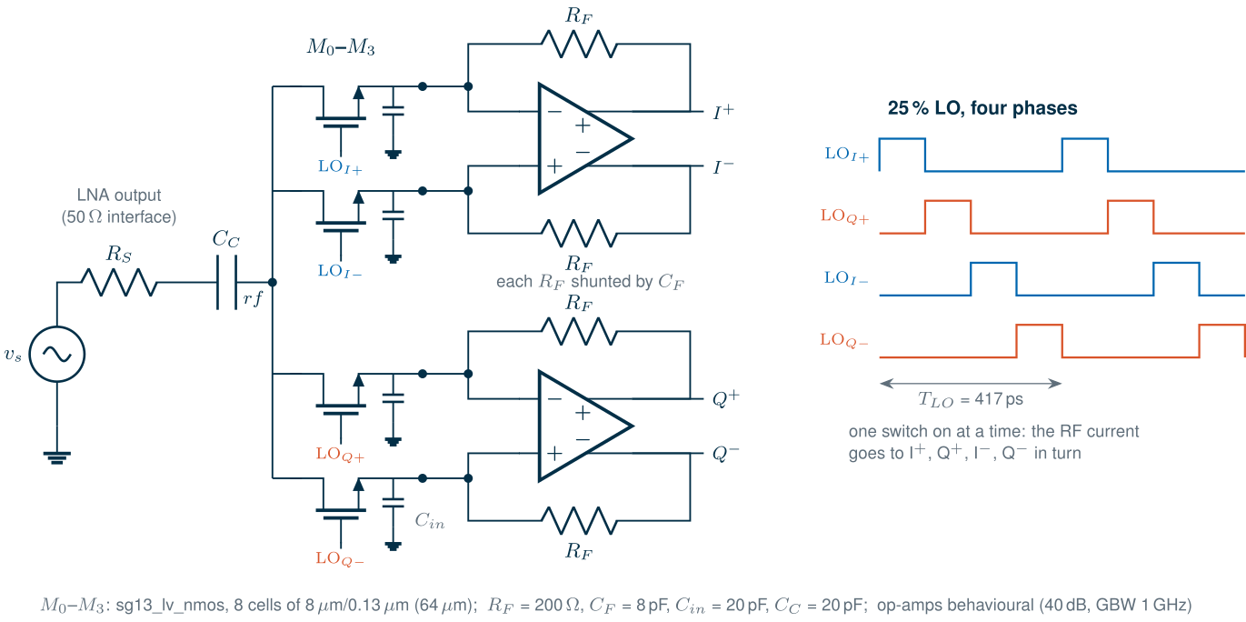
With ideal switches of on-resistance \(R_{sw}\) and an ideal virtual ground, exactly one switch conducts at a time, so the RF current is \(v_s/(R_S + R_{sw})\) whatever the LO phase. The I output collects it through the mixing function \(p_0(t) - p_2(t)\) (the I+ pulse minus the I− pulse), whose fundamental is \(2a_1 = 2\sqrt2/\pi\). The conversion gain against the available source voltage follows:
Key equation · Gain of the 25 % current-mode passive mixer
\[G = \frac{2\sqrt{2}}{\pi}\,\frac{R_F}{R_S + R_{sw}} \tag{10.3}\]For the course design, \(R_F\) = 200 Ω and \(R_{sw}\) = 20.6 Ω give +8.13 dB.
50 % against 25 % duty cycle
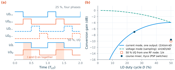
A single differential mixer with a 50 % LO has the larger current gain, \(2/\pi\) against \(\sqrt2/\pi\) for 25 % (−3.92 against −6.93 dB, Eq. 10.2). An I/Q pair fed from one RF node changes the picture (Figure 10.2a). With 50 % LOs, an I switch and a Q switch are always on together, so the RF current splits between the I and Q TIAs: each gets half, \(1/\pi\) (−9.94 dB), and each TIA’s noise and signal leak into the other path through the shared node. With 25 % phases only one switch is on at a time, every TIA gets the whole current while its switch conducts, and the I/Q pair gains 3 dB [117, 116]. In a voltage-mode passive mixer, which drives a high impedance and samples the RF voltage on a capacitor, the gain rises as the window narrows, \(\sin(\pi D)/\pi D\): the familiar \(2\sqrt2/\pi\) (−0.91 dB) of a 25 % double-balanced voltage-mode mixer against \(2/\pi\) (−3.92 dB) at 50 %.
Switch sizing and LO power
A wider switch lowers \(R_{sw}\), which raises the gain for a given \(R_F\), lowers the switch’s own noise and makes the switch more linear; but its gate capacitance must be charged by the LO buffer every period. Xyce’s PSP model of an 8 µm sg13_lv_nmos cell at \(V_{GS}\) = 0.9 V gives 1320 Ω·µm of on-resistance and an effective gate capacitance (gate charge over the 1.2 V swing) of 1.24 fF/µm. The course switch, eight cells (64 µm), has \(R_{sw}\) = 20.6 Ω and \(C_g\) = 79.6 fF; its eight cells divide SG13G2’s fixed 40 Ω gate resistance per RF cell to 5 Ω. (Our Xyce runs use the PSP core model, rfmode=0, with that 5 Ω added as an explicit gate resistor. For one on cell at 2.4 GHz, the drain conductance agrees with ngspice’s rfmode=1 model to 0.02 %, and its drain susceptance is 5.7 % lower. Xyce also accepts rfmode=1 directly, in which case the explicit resistor must be left out.) Four such gates switched at 2.4 GHz from 1.2 V, with a fan-out-of-four buffer chain adding a third, need
The 25 % phases come from the Chapter 13 divide-by-two. Its I and Q outputs, converted to CMOS levels, feed four NAND gates, each followed by one inverter that drives a switch: \(\mathrm{LO}_{I+} = \overline{\mathrm{NAND}(I, \overline{Q})} = I\cdot\overline{Q}\), and so on. A 25 % pulse at 2.4 GHz lasts 104 ps, only a few gate delays in this process, so the chain must be short. Our first version, a NOR gate and two inverters of fan-out four, swallowed the pulse: the NOR’s series pMOS gave it a slow rising edge, three stage delays did the rest, and the switch gates never rose above 0.7 V (Xyce). The two-stage chain of Figure 10.3a works. It has NAND gates of 8/8 µm and inverters of 12/24 µm (nMOS/pMOS, L = 0.13 µm), fed by ideal 50 % I/Q square waves with 30 ps edges. The switch gates swing fully, with 40.7 ps rise and 36.0 ps fall times (10–90 %). Each switch stays above its turn-on voltage (0.803 V, where it reaches 5 % of its on-conductance) for 26.4 % of the period, so at each LO edge two switches conduct together, weakly, for 5.7 ps. The chain draws 2.73 mW, 1.9 times Eq. (10.4), not counting the converters that drive the NAND inputs. The inverters’ own capacitance and the short-circuit current during edges of 40 ps cost more than the third that Eq. (10.4) allowed.
One detail of the gates’ wiring matters. A NAND’s two nMOS are stacked, and a pulse that starts at the top input has a different edge from one that starts at the bottom input. If the I pulses start at the top input and the Q pulses at the bottom one, I and Q differ: the mixer driven by such a chain has an I/Q gain error of 0.72 dB and a phase error of 1.15°, more than the whole receiver’s 0.2 dB budget. Stacking the inputs so that every pulse starts at the top input (I with \(\overline{Q}\), Q with I, \(\overline{I}\) with Q, \(\overline{Q}\) with \(\overline{I}\)) makes the four pulses identical, and the errors fall to 0.0002 dB and 0.005°.
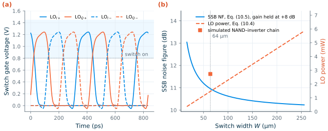
The divider’s quadrature error (0.114° per millivolt of input offset, Chapter 13) passes straight into the edges of the 25 % pulses, so it remains the main source of I/Q phase error. In Eq. (10.5) below, \(R_{sw}\) enters only through \(R_S + R_{sw}\) and the switch term. Beyond the point where \(R_{sw}\) is small against \(R_S\), a wider switch buys little noise for proportionally more LO power (Figure 10.3b). With the gain held at +8 dB, the hand-analysed noise figure falls from 13.0 dB at 16 µm to 11.0 dB at 64 µm, but only to 10.5 dB at 128 µm, where Eq. (10.4) already asks for 2.93 mW.
Impedance transparency
A passive mixer conducts in both directions, so the TIA’s input impedance appears, translated to around \(f_{LO}\), at the RF port: the mixer is transparent [116]. For the current-mode design the TIA holds a near-zero impedance over the IF band, and the RF port sees little more than \(R_{sw}\): the simulated input impedance at 2.401 GHz is 28.0 − j3.0 Ω. That low impedance is what makes the current-mode mixer linear: the RF voltage across the switches stays small, so their gate overdrive hardly changes with the signal. The same property, with capacitors instead of TIAs, gives the N-path filters of Section 10.6.
10.4 Active mixers and the Gilbert cell
An active mixer first converts the RF voltage to a current in a transconductor, then commutates that current with a pair of switching transistors into a load. The single-balanced version has one transconductor and one switching pair; the Gilbert cell [115] (Figure 10.4) uses a differential transconductor and a quad of switches cross-coupled so that both the RF and the LO feedthrough cancel at the output. With square-wave switching its gain against the available source voltage, for a gate driven directly by the source, is \(G = (4/\pi)\,g_mR_L\).
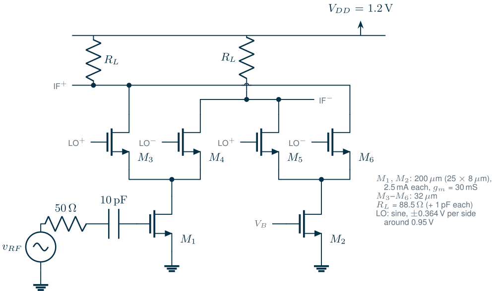
Its weaknesses are the ones the passive mixer avoids. The transconductor, a common-source pair, sets the linearity, exactly as in Chapter 4’s stages. The switching pair is briefly balanced at each LO crossing, and during those moments its own noise reaches the output; and its flicker noise, which a passive switch without DC current does not have, appears at the IF through the shift of the crossing instants [118]. Darabi and Abidi’s model gives, for white noise,
Key equation · SSB noise factor of a Gilbert cell (white noise)
\[F_{SSB} \approx \frac{\pi^2}{4}\left(1 + \frac{2\gamma}{g_mR_S}\right) + \frac{2\pi^2}{4g_m^2R_LR_S} + \frac{2\pi\gamma I_D}{A_{LO}\,g_m^2R_S} \tag{10.8}\]source and transconductor, load, and the switching quad during its transitions; \(A_{LO}\) is the differential LO amplitude and \(I_D\) the current of each transconductor device.
For a Gilbert cell with the same +8 dB gain, \(g_m\) = 30 mS per side (\(I_D\) = 2.5 mA at \(g_m/I_D\) = 12 S/A), \(R_L\) = 66 Ω, \(\gamma\) = 1 and the Chapter 13 LO swing of ±0.728 V, Eq. (10.8) gives an SSB noise figure of 9.08 dB before flicker noise, at 6.0 mW of DC power. The transconductor term alone is 3.41, as large as the source’s own π²/4: a Gilbert cell’s noise is bought with transconductance, and its transconductance with current. Flicker noise of the switches adds to this at a 1 MHz IF.
We checked the estimate by simulating such a cell (Xyce and ngspice, PSP). Its transconductors are 200 µm wide (25 cells of 8 µm, L = 0.13 µm), so that 2.5 mA gives the assumed \(g_m\) = 30.0 mS (\(g_m/I_D\) = 12 S/A); its switches are 32 µm; its LO is a sine with the Chapter 13 swing, ±0.364 V on each side around 0.95 V. A sine LO commutates the current less sharply than a square wave: the simulated gain is 0.743 of \((4/\pi)g_mR_L\), so \(R_L\) = 88.5 Ω is needed for +8.00 dB. With that efficiency and the PSP model’s device noise (\(\gamma\) = 0.91 for the transconductor), Eq. (10.8) gives 9.39 dB for white noise alone. The switches’ flicker noise, though, has a corner at 15.5 MHz in these short devices, and at a 1 MHz IF it adds 3.47 to the noise factor: 10.9 dB, no better than the passive mixer. The linearity is worse: two tones at −20 dBm extrapolate to an IIP3 of +0.3 dBm, below the budget’s +4 dBm (−2.3 dBm from tones at −12 dBm). The cell draws 7.4 mW from the 1.2 V supply, against 6.0 mW from the two bias currents alone.
10.5 Linearity and port-to-port isolation
Third-order distortion. In the passive mixer the switches are the only nonlinear devices (the TIA here is a linear behavioural model; Section 10.8 repeats the test with the transistor-level op-amp). Their on-resistance depends on \(V_{GS}\), and the source of a switch moves with the RF voltage across it. Because the current-mode mixer keeps that voltage small, its IIP3 is high. We applied two tones at LO + 3 MHz and LO + 5 MHz, whose third-order product falls at 1 MHz, the wanted IF, as in BLE’s intermodulation test.
Second-order distortion. A perfectly symmetric mixer has no IM2 at its differential outputs: the low-frequency currents that the switches’ nonlinearity produces flow equally into I+ and I−. Mismatch breaks the symmetry, and in a low-IF receiver the IM2 of two interferers 1 MHz apart, or the envelope of one amplitude-modulated interferer, lands in the channel (Section 5.5). We gave one switch a deliberate 1 % excess width and measured the IM2 at 2 MHz (the difference of the two tones).
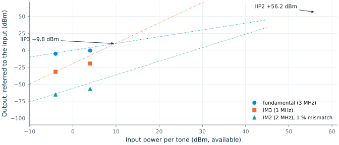
Figure 10.5 shows the result at three powers per tone, with switch M0 one percent wider than the others. Between −16 and −4 dBm the IM3 product grows with a slope of 3.00, and the −16 dBm point extrapolates to an IIP3 of +9.8 dBm (+9.3 dBm from −4 dBm). The IM2 product grows faster than the textbook slope of 2 (3.07), so the intercept depends on where it is read: +70.1 dBm from −16 dBm, +56.2 dBm from −4 dBm; we quote the lower, IIP2 = +56.2 dBm. The mixer compresses early: referred to the input, its fundamental is 1.13 dB below the small-signal value at −4 dBm and 4.35 dB at +4 dBm. With two tones of −4 dBm from a 50 Ω source the RF node swings by about a quarter of a volt, enough to modulate the switches’ 0.9 V of gate overdrive: the low input impedance protects the switches only while the source cannot push much voltage into it. The 1 % mismatch leaves a DC offset of −0.48 mV at the I output at −4 dBm (−0.081 mV at −16 dBm), and I/Q errors of 0.023 dB and 0.006°. These runs used \(R_F\) = 200 Ω. Repeated at 220 Ω (Section 10.8), the test gives an IIP3 of +9.9 dBm from −16 dBm, an IIP2 of +56.0 dBm from −4 dBm and 1.14 dB of compression at −4 dBm: the TIA’s gain does not change the switches’ linearity.
Feedthrough and DC offsets. With matched switches, the four LO phases couple through the gate-drain capacitances into the RF node with phases 0°, 90°, 180° and 270°, and their sum cancels at \(f_{LO}\); at \(4f_{LO}\) they add. Any mismatch leaves a residue at \(f_{LO}\) that travels back through the LNA to the antenna (LO–RF feedthrough) and, reflected, mixes with the LO itself: self-mixing produces a DC offset at the output. In a zero-IF receiver that offset sits on the signal; in the course’s low-IF receiver it lies 0.5 MHz below the channel, where a high-pass corner of tens of kilohertz removes it (Table 5.1). With the transistor-level LO chain of Figure 10.3, the LO power delivered back into the 50 Ω source at \(f_{LO}\) is −68.7 dBm with matched switches and −78.0 dBm with M0 1 % wider. The two residues partly cancel, so the matched chain itself is not perfectly symmetric, but either way the leakage stays below −68 dBm. At \(4f_{LO}\), where the four edges add, the leakage is −34.3 dBm, which the LNA’s reverse isolation and the band filter must keep from the antenna. LO–IF feedthrough is filtered by \(C_{in}\) and \(C_F\): in the simulation the residual LO at one TIA output is −73.5 dBV.
10.6 N-path filters and mixer-first receivers
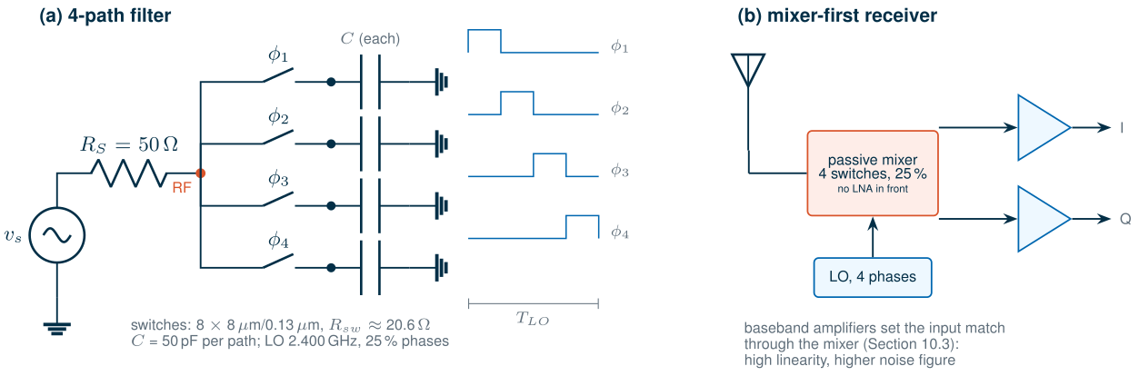
Replace the four TIAs by four capacitors and the passive mixer becomes a 4-path filter (Figure 10.6a): each capacitor, connected to the RF node for a quarter period, charges to the average RF voltage in its window. For a signal near \(f_{LO}\) the capacitors hold a slowly varying baseband copy of it, and the switches convert that copy back up; far from \(f_{LO}\) the capacitors average the signal to nothing and short the RF node through \(R_{sw}\). The capacitors’ low-pass response, with the time constant \(N(R_S + R_{sw})C\) of a capacitor that is connected only one \(N\)-th of the time, is translated to a band-pass response centred on the LO and tuned by it [119]. Two numbers bound it: the stop-band floor \(R_{sw}/(R_S + R_{sw})\), set by the switch, and a centre loss from the harmonics that the switched waveform dissipates in \(R_S\), a shunt resistance of \(4.27\,(R_S + R_{sw})\) for four paths [116].
Key equation · Bandwidth and stop band of an N-path filter
\[\Delta f \approx \pm\frac{1}{2\pi N(R_S + R_{sw})C}, \qquad \left.\frac{v_{rf}}{v_s}\right\vert_{\lvert f - f_{LO}\rvert \gg \Delta f} = \frac{R_{sw}}{R_S + R_{sw}} \tag{10.7}\]\(\Delta f\) is the half-width of the pass band around \(f_{LO}\), for \(N\) paths with capacitance \(C\) each.
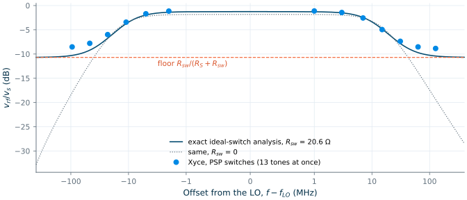
With the course switches the floor is only \(20.6/70.6\), −10.7 dB, and 50 pF per path gives a half-width of 11.3 MHz. Figure 10.7 checks both numbers with a transient of the PSP switches and 13 tones applied at once, from 95 MHz below to 127 MHz above the LO. Near the LO the simulation follows the exact ideal-switch analysis (a piecewise-exponential solution over one LO period, in the chapter script): −1.12 dB at +1 MHz against −1.28 dB. The loss comes from the harmonics; even switches with \(R_{sw}\) = 0 would lose 1.82 dB. Far from the LO the PSP switches do worse than the ideal floor: −8.9 dB at +127 MHz and −7.8 dB at −95 MHz. The exact analysis meets the simulated stop band at +127 MHz with \(R_{sw}\) = 27.5 Ω, close to the course mixer’s simulated 28 Ω input resistance (Section 10.8). During the LO edges each switch passes through high resistance, and the stop band sees the time average. An N-path filter for blocker rejection needs switches several times wider, with sharper edges.
Mixer-first receivers (Figure 10.6b) take the idea further: they put the passive mixer directly at the antenna, set the input match by the baseband impedance through the transparency of Section 10.3, and accept a higher noise figure for very high linearity [116]. The course radio keeps an LNA in front (Chapter 9), because its 8 dB system NF leaves no room for a mixer-first front end’s noise.
10.7 Quadrature LO generation
The course LO chain is short: the CML divide-by-two of Chapter 13 produces I and Q at 2.4 GHz with a differential swing of ±0.728 V and a quadrature error of 0.114° per millivolt of offset at its input; a CML-to-CMOS converter brings them to rail-to-rail levels, and the NAND gates of Section 10.3 make the four 25 % phases. The edges of each 25 % pulse are the edges of I and Q themselves, so the pulses are as accurate as the divider. The alternatives cost more. An RC–CR or polyphase filter makes quadrature from a single-phase LO with passive components, but only exactly at one frequency and with a loss that the LO buffers must make up [81]; a quadrature VCO couples two oscillators and trades phase noise for phase accuracy. Dividing a VCO at twice the LO, the course choice of Chapter 5, gives wide-band quadrature for the price of a VCO at 4.8 GHz.
10.8 The course I/Q mixer
Simulation setup
The course mixer of Figure 10.1 was simulated in Xyce, whose PSP plugin ran these SG13G2 transients about forty times faster than ngspice’s OSDI model on our machine (the same 10 ns switch transient: 0.5 s against 21 s). The LO is an ideal 25 % four-phase pulse source, 0 to 1.2 V with 25 ps edges, at 2.400 GHz; the wanted tone lies 1 MHz above it. The TIAs are behavioural: a fully differential op-amp with 40 dB of gain and a single pole at 10 MHz (1 GHz gain-bandwidth), and ideal output stages. Their linearity and swing therefore do not limit these results; the subsection The TIA’s op-amp below replaces them by a transistor-level OTA and repeats the gain, noise and two-tone simulations.
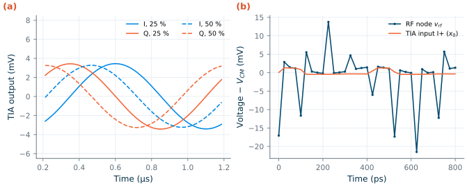
The simulated conversion gain is +7.18 dB, 0.95 dB below Eq. (10.3). The difference is the input resistance: the RF port presents 28.0 − j3.0 Ω instead of \(R_{sw}\) = 20.6 Ω, because during the LO edges the switch resistance rises and for a few picoseconds no switch conducts fully, and the TIA’s virtual ground is not perfect; \(20\log_{10}[(R_S + R_{sw})/(R_S + 28)]\) accounts for −0.87 dB of it. Referred to the RF current, the current conversion gain is −6.99 dB against −6.93 dB from Eq. (10.2). With a 50 % LO the current gain falls to −9.51 dB, near the −9.94 dB of I and Q sharing the current, but the voltage gain only to 6.73 dB: with two switches on at once the input resistance drops to 11.5 Ω and the 50 Ω source delivers more current. The 25 % mixer keeps the larger gain and, more importantly, independent I and Q paths. With matched switches the I and Q outputs differ by 0.0001 dB and 0.012° from quadrature (Figure 10.8a), the numerical floor; the I/Q accuracy of the mixer is set by mismatch and by the LO, not by the topology.
The budget asks for +8 dB, so the design raises \(R_F\) to 220 Ω (223 Ω with the transistor-level op-amp of the subsection The TIA’s op-amp); \(C_F\) stays at 8 pF. Simulated again, the mixer gives +8.02 dB, where scaling the 200 Ω result by \(R_F\) predicted +8.01 dB, with an input impedance of 28.4 − j3.0 Ω and I/Q errors of 0.013 dB and 0.009°. Driven by the transistor-level LO chain of Figure 10.3 instead of ideal pulses, the gain is +8.20 dB: the slower edges let two switches conduct together for a few picoseconds, which lowers the input resistance to 26.1 Ω and lets the source deliver more current. Table 10.2 quotes the ideal-LO value, the condition of every other simulation in this chapter.
Noise figure
Neither simulator has a periodic noise analysis (Chapter 2). We therefore start from the LPTV analysis of Section 10.3, with ideal switches of resistance \(R_{sw}\), and then check it by simulation. The source noise in all sidebands gives π²/4; the switches add the same factor times \(R_{sw}/R_S\); the two feedback resistors add \(2\cdot4kTR_F\) at the output; and the op-amp’s input noise \(e_n\) reaches the output with a noise gain of \(1 + R_F/4(R_S + R_{sw})\), since each TIA input sees the source through its switch one quarter of the time:
Key equation · SSB noise factor of the 25 % current-mode mixer
\[F_{SSB} = \frac{\pi^2}{4}\left(1 + \frac{T}{T_0}\frac{R_{sw}}{R_S}\right) + \frac{T}{T_0}\,\frac{\pi^2 (R_S+R_{sw})^2}{R_SR_F} + \frac{\overline{e_n^2}\,\left(1 + \frac{R_F}{4(R_S+R_{sw})}\right)^2}{4kT_0R_S\,\frac{2}{\pi^2}\,\frac{R_F^2}{(R_S+R_{sw})^2}} \tag{10.5}\]
For the op-amp we assume an input pair with \(g_m\) = 20 mS per device and \(\gamma\) = 1, \(e_n\) = 1.29 nV/√Hz differential. At \(R_F\) = 200 Ω the four terms are 2.47, 1.05, 5.09 and 3.71: the feedback resistors contribute 41 % of the noise factor and the op-amp 30 %, the source itself only 20 %. The SSB noise figure is 10.9 dB, and 7.9 dB after image rejection, Eq. (10.6); at 220 Ω it is 10.6 dB. The analysis ignores the switch transitions and the op-amp’s flicker noise.
Transient noise. In a transient, ngspice draws noise only from the trnoise sources we add, not from the PSP model (Section 2.6). The noise run therefore uses behavioural switches. Each is a conductance \(g(V_G) = ks\ln\!\left(1 + e^{(V_G - V_t)/s}\right)\) fitted to the PSP switch (within 4.2 % above 0.8 V), and the RF node carries the 173 fF that the four PSP switches put on it (Xyce: 163 fF with all four off, 182 fF with one on). Every noise source is a trnoise source with a new sample every 10 ps: \(4kTg(t)\) across each switch, \(4kT/R_F\) across each feedback resistor, \(e_n\) at each op-amp input and \(4kT_0R_S\) in series with the source. Six copies of the mixer share one netlist and one LO. Each has a 3 mV tone at LO + 1 MHz for its own gain and one set of noise sources switched on: the source, the switches, the feedback resistors or the op-amp alone, all four at \(R_F\) = 200 Ω, and all four at 220 Ω. The record is 40 µs long (100 minutes of simulation on the shared machine), averaged in 2 µs segments over 0.5–10 MHz. With every source on, the SSB noise figure at \(R_F\) = 220 Ω is 11.5 ± 0.15 dB, and 8.65 dB after image rejection (Figure 10.9a): about 0.9 dB above Eq. (10.5). Such a run scatters more than its length suggests. The I and Q outputs of one copy, or the four quarters of its record, differ by up to 1 dB, and the ± values here come from that spread. At 200 Ω the copy with every source on gives 12.3 ± 0.3 dB, while the four copies with one source each add up to 11.8 dB.
A check without scatter. A transient-noise result has statistical scatter, and it cannot say which assumption of Eq. (10.5) is wrong. For a circuit that is linear but periodically time-varying there is an exact method, the periodic small-signal analysis of commercial RF simulators [32]. Such a circuit couples only the frequencies \(f + nf_{LO}\), so its response to a small signal or a noise source at all sidebands, here \(n\) = −40 to 40, is one linear system: the harmonic transfer (or conversion) matrix. The thermal noise of a switch is cyclostationary: its components one LO harmonic apart are correlated, through the Fourier coefficients of \(g(t)\). The chapter script solves this system for the same circuit in Python (tools/figs/_ch10_lptv.py), in a fraction of a second per frequency. It gives 11.57 dB at 200 Ω and 11.25 dB at 220 Ω (8.24 dB after image rejection), with a noise figure that stays within 0.06 dB from 0.25 to 10 MHz. The single-source transient copies lie 1–9 % above its four terms, and the copies with every source on 0.3–0.7 dB above its totals, about twice their scatter. We take the periodic analysis as the simulated value of the design and the transient runs as its check.
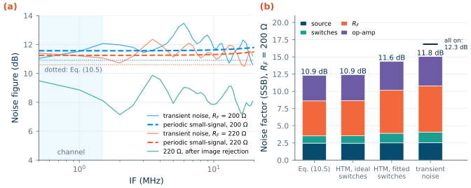
Figure 10.9b separates the causes. With ideal switches the periodic analysis gives 10.94 dB, 0.03 dB from Eq. (10.5): the hand analysis is right about the circuit it assumes. What it leaves out is the switch transitions. With the fitted switches and 25 ps LO edges, the gain falls from 7.97 to 7.11 dB (7.18 dB with PSP switches in Xyce), and the input resistance rises from 21 to 29 Ω, because at every edge the conducting switch passes through high resistance. Referred to the input through the smaller gain, the feedback resistors’ noise grows by 22 %, the op-amp’s by 12 % and the switches’ own by 29 %. Together these raise the SSB noise figure by 0.63 dB. Two smaller effects lie inside the transient run’s scatter: the RF-node capacitance moves the noise figure by 0.06 dB, and the trnoise sources, whose density rolls off as \(\mathrm{sinc}^4\) above about 10 GHz, under-represent the noise folded from the LO harmonics by 0.02 dB. Eq. (10.5) with the simulated 28 Ω input resistance in place of \(R_{sw}\) gives 11.55 dB at 200 Ω and 11.23 dB at 220 Ω, within 0.02 dB of the periodic analysis: a good shortcut.
The op-amp’s own devices. The analysis and the simulation both give the op-amp the white input noise of an ideal pair, 1.29 nV/√Hz. Real SG13G2 devices are noisier. Sized for the assumed \(g_m\) = 20 mS at \(g_m/I_D\) = 15 S/A (1.33 mA each), a pMOS input device of L = 1 µm is 2.6 mm wide; the PSP model gives it \(\gamma\) = 1.36 and a flicker corner at 198 kHz (ngspice .noise). Averaged over the 0.5–1.5 MHz channel, the pair’s input noise is 1.66 nV/√Hz. That raises the op-amp’s term at \(R_F\) = 220 Ω from 3.75 to 6.2 and the SSB noise figure from 11.25 to 12.0 dB, the budget’s limit; the white noise alone accounts for 0.4 dB of that. With L = 0.5 µm (1.36 mm wide) the corner rises to 706 kHz and the noise figure to 12.7 dB. The mixer’s real noise problem is therefore its op-amp’s input pair, which must be long and wide and still fast enough to hold the virtual ground. The subsection The TIA’s op-amp below designs that op-amp and replaces this estimate by the noise of a complete OTA.
What this means for your design
In a current-mode passive mixer driven from 50 Ω, the TIA, not the switches, sets the noise. A low-resistance source forces a small \(R_F\) for a given gain, so \(R_F\)’s own noise is large compared with the converted source noise, and the op-amp’s noise is amplified by \(1 + R_F/4(R_S+R_{sw})\). Driving the mixer from a high-impedance transconductance LNA (an LNTA) allows a larger \(R_F\) and lowers both terms; this is why many receivers pair a passive mixer with a current-output LNA. The switches matter through their edges more than through their on-resistance: slow edges cost gain, and every noise term downstream is referred to the input through that gain.
The TIA’s op-amp
Every result so far uses a behavioural op-amp: its power, about 13 mW for the two TIAs, was an estimate, and its noise came from single devices. This subsection designs it in SG13G2 and puts it into the mixer. The method is that of The Art of Analog IC Design, Chapter 12 [4]: choose each device’s \(g_m/I_D\) and length, then read its width from a table of current density (here a DC sweep of one 40 µm cell of each device type, in tools/figs/_ch10_ota.py).
What the TIA asks for. No DC current flows in \(R_F\), so each TIA’s inputs and outputs share one DC level, the switches’ 0.3 V. Inputs that close to ground need a pMOS input pair, and the outputs must swing around 0.3 V. Each output drives \(R_F\) into a virtual ground, so the output stage must supply milliamperes: in the −16 dBm two-tone test of Section 10.5 each output moves by about ±0.13 V, ±0.6 mA in 220 Ω. The loop gain at 1 MHz should match the behavioural op-amp’s 35.3 dB, which the +8.02 dB already includes. And with the other terms of the periodic analysis unchanged, the 12 dB budget leaves the op-amp an input noise of 1.66 nV/√Hz averaged over the channel, flicker noise included.
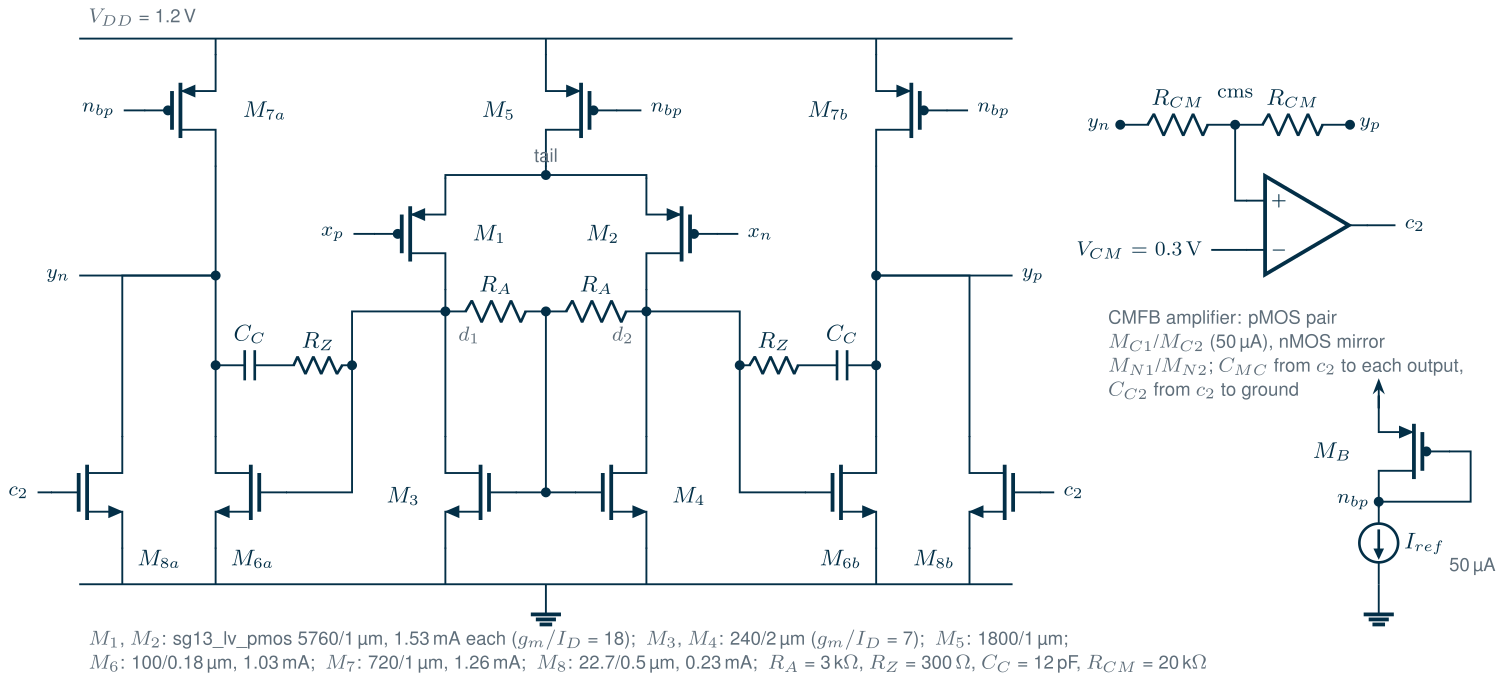
tools/figs/_ch10_ota.py). $$R_A$$ makes the loads M3/M4 diode-connected for the common mode; the output CMFB acts on the pull-downs M8, so the TIA has no latched state. RF goes from yp to xp and from yn to xn (Figure 10.1). Capacitors and resistors ideal; one OTA draws 5.67 mA.The circuit. Figure 10.10 is a fully differential two-stage Miller OTA. The input pair M1/M2 is 1 µm long, against flicker noise, with its bulk tied to the common source. For \(g_m\) = 27.5 mS at \(g_m/I_D\) = 18, each device is 5.76 mm wide and carries 1.53 mA. The nMOS loads M3/M4 run at \(g_m/I_D\) = 7 with L = 2 µm, so that their noise current, \(4kT\gamma g_{m3}\), stays well below the pair’s. Their gates sit at the midpoint of two 3 kΩ resistors \(R_A\) between the first-stage outputs: the loads are diode-connected for the common mode, which holds the first stage’s outputs at 0.49 V, and current sources for the difference. The second stage is the nMOS M6 (100 µm/0.18 µm, 1.03 mA, \(g_m/I_D\) = 12.7) with the pMOS current source M7. \(C_C\) = 12 pF with \(R_Z\) = 300 Ω compensates it; \(R_Z\), well above \(1/g_{m6}\), puts the compensation zero in the left half-plane at 59.5 MHz, near the crossover, where it adds phase. A common-mode feedback (CMFB) loop senses the outputs through two 20 kΩ resistors, compares their average with 0.3 V and drives M8, a pull-down that carries a fifth of the output current. One OTA draws 5.67 mA from 1.2 V, 6.81 mW.
Two versions that failed. The first version let the CMFB act on the first-stage loads, a common choice. The TIA then had a second DC solution, with its outputs at the supply. If the outputs rise, the inputs follow them through \(R_F\) until the pMOS pair turns off; the loads then pull the first stage down, M6 turns off, and nothing pulls the outputs down again. A pull-down at the outputs removes this latch, because M8 conducts whatever the first stage does. The second version had \(R_A\) = 20 kΩ. With the large gates of M3/M4 behind 10 kΩ, the first stage’s common mode followed too slowly, the common-mode loop through \(R_F\) and the input pair lost its phase margin, and the TIA’s outputs oscillated between 0.02 and 1.09 V after power-up. With 3 kΩ the power-up settles at 0.299 V, for a small loss of first-stage gain.
Simulated alone. The OTA matches the behavioural op-amp where the mixer needs it (Figure 10.11a, Table 10.1). With the mixer’s source in place, about \(4(R_S + R_{in})\) = 313 Ω per side at the IF, the TIA’s loop gain is 35.2 dB at 1 MHz, against the behavioural 35.3 dB, and it crosses unity at 54.7 MHz with 62° of phase margin. With all switches open the source is gone, the feedback factor is largest and the margin falls to 56°. The loop cannot cross much higher: above a few megahertz the capacitance on the TIA inputs takes over from the source, and the feedback factor falls toward \(C_F\) over the total input capacitance. Most of that capacitance is the OTA’s own: 103 pF per side at 1 MHz, a third of it the pair’s gate capacitance and the rest its gate–drain capacitance multiplied by the first stage’s gain. At the IF it costs almost nothing: the inputs are a virtual ground, and the source impedance next to it is five times smaller. The CMFB loop crosses unity at 8.2 MHz with 64° of margin.
The input noise (Figure 10.11b) is 1.45 nV/√Hz white, with a flicker corner at 186 kHz, and 1.57 nV/√Hz averaged over the channel. That is 1.48 times the behavioural op-amp’s noise power, but inside the 1.66 nV/√Hz that the budget allows. The input pair produces 75 % of it (9 percentage points of that as flicker noise), the loads 23 % (8 points flicker), and the second stage and the CMFB the remaining 2 %. The outputs stay within 1 dB of the small-signal transimpedance over ±0.39 V differential; the limit is the output that swings toward ground, because both outputs start only 0.3 V above it. Pelgrom’s law with the SG13G2 threshold mismatch of the sibling course (3.0 mV·µm for pMOS, 5.7 mV·µm for nMOS; The Art of Analog IC Design, Chapter 13) gives an input offset of σ = 0.11 mV, negligible next to the mismatch offsets of Section 10.5.
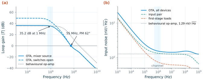
.noise, outputs loaded by $$R_F \parallel C_F$$), and the shares of the input pair and the first-stage loads. Shaded: the 0.5–1.5 MHz channel.Table 10.1. The TIA's op-amp: the behavioural model of the earlier simulations against the transistor-level OTA of Figure 10.10 (SG13G2, tt, 27 °C, TIA with RF = 220 Ω, CF = 8 pF, Cin = 20 pF).
| Quantity | Behavioural op-amp | Transistor-level OTA | Method |
|---|---|---|---|
| Loop gain at 1 MHz, mixer source | 35.3 dB | 35.2 dB (43.2 dB, switches open) | ngspice AC, double injection |
| Loop crossover, phase margin | 295 MHz, 83° | 54.7 MHz, 62° (56°, switches open); gain margin 13.5 dB | ngspice AC |
| CMFB loop crossover, phase margin | — (ideal) | 8.2 MHz, 64° | ngspice AC |
| Open-loop gain, outputs loaded by \(R_F \parallel C_F\) | 40 dB, pole at 10 MHz | 35.7 dB, pole at 3.26 MHz | ngspice AC |
| Input noise: white; channel average | 1.29; 1.29 nV/√Hz | 1.45; 1.57 nV/√Hz (corner 186 kHz) | ngspice .noise |
| Output range (1 dB), differential | unlimited | ±0.39 V | ngspice DC |
| Input offset, σ | 0 | 0.11 mV | Pelgrom’s law |
| Supply power, one OTA | about 6.4 mW (estimate) | 6.81 mW (5.67 mA) | ngspice operating point |
In the mixer. With the OTA in both TIAs (Xyce, PSP switches and OTAs, ideal LO) and \(R_F\) = 220 Ω, the mixer gives +7.90 dB, 0.12 dB below the behavioural TIA; the periodic analysis, with the OTA entered as its simulated four-port admittance, predicts a drop of 0.10 dB. The final design therefore raises \(R_F\) to 223 Ω, which gives +8.05 dB. The input impedance, 28.4 − j2.9 Ω, hardly changes, and the I/Q errors with matched switches stay small, 0.025 dB and 0.11°. The two OTAs draw 13.6 mW in the transient, 6 % more than the 12.8 mW estimate.
For the noise figure, _ch10_lptv.py stamps the OTA’s four-port admittance into the harmonic transfer matrix at every sideband and applies its simulated input noise at the IF; at the LO harmonics the OTA has no gain and \(C_{in}\) shorts its inputs. At \(R_F\) = 220 Ω the SSB noise figure is 11.88 dB at 1 MHz and 11.93 dB averaged over the channel; the op-amp’s term grows from 3.75 to 5.75 and that of \(R_F\) from 5.68 to 5.94. The final 223 Ω lowers both terms a little, to 5.65 and 5.85: the noise figure is 11.84 dB at 1 MHz and 11.88 dB averaged over the channel, from 12.09 dB at 0.5 MHz, where the flicker noise is largest, to 11.75 dB at 1.5 MHz; after image rejection it is 8.87 dB. That is 0.63 dB above the behavioural op-amp’s 11.25 dB and 0.11 dB below the 12.0 dB estimated earlier from an input pair alone: the OTA’s loads add about what its larger, longer pair saves. The mixer meets the 12 dB budget, with 0.12 dB to spare.
The two-tone test with the OTA (switch M0 1 % wider, as in Section 10.5) at 220 Ω gives an IIP3 of +11.1 dBm from −16 dBm and +11.0 dBm from −22 dBm (IM3 slope 2.96), against +9.9 dBm with the behavioural TIA: the OTA does not degrade it at these levels. At −10 dBm per tone the lower output swings down to 62 mV, the gain compresses by 0.43 dB and the extrapolation gives only +5.0 dBm. The IM2 product does not grow with a slope of 2 (it stays between 15 and 42 µV at the I output from −22 to −10 dBm), so its intercept is ill-defined; the lowest value, +41.5 dBm from −22 dBm, still clears the +35.3 dBm budget by 6 dB. At the final 223 Ω the IIP3 from −16 dBm is +10.6 dBm and the IIP2 +58.4 dBm. Two tones of −4 dBm, which compressed the behavioural TIA by 1.14 dB, overload the OTA: its outputs swing from 44 mV to 0.54 V and the gain drops by 4.74 dB. A single tone at LO + 1 MHz, swept from −16 to 0 dBm, compresses the gain by 0.68 dB at −4 dBm and 2.0 dB at −2 dBm: the input-referred 1 dB compression point is −3.5 dBm (available power, interpolated). With outputs that sit only 0.3 V above ground on a 1.2 V supply, the TIA, not the switches, now sets the mixer’s large-signal limit.
What is still assumed. The OTA’s capacitors and resistors are ideal, without the MIM and poly models and their parasitics (Xyce loads only the PSP model), its 50 µA reference is an ideal current source, and it has no layout. All OTA results are for the typical corner at 27 °C. The noise figure with the OTA comes from the periodic small-signal analysis with behavioural switches and an ideal LO; no transient-noise run includes the OTA’s devices, because ngspice’s transient analysis draws no noise from the PSP model. The source is still the 50 Ω interface, not the designed LNA.
Results against the budget
Table 10.2. The course I/Q mixer against its Table 5.3 budget (50 Ω source, 2.400 GHz LO, IF 1 MHz, RF = 220 Ω with the behavioural op-amp and 223 Ω with the transistor-level OTA, tt, 27 °C), and the simulated Gilbert cell at the same gain.
| Quantity | Budget (Table 5.3) | Course mixer (25 % passive + TIA) | Method | Pass? | Gilbert cell |
|---|---|---|---|---|---|
| Conversion gain | +8 dB | +8.02 dB (+8.20 dB with the transistor-level LO chain); with the transistor-level OTA +7.90 dB at 220 Ω and +8.05 dB at 223 Ω | Xyce transient | pass | +8.00 dB (Xyce) |
| SSB noise figure | ≤ 12 dB | 11.25 dB with the behavioural op-amp (periodic small-signal; transient noise 11.5 ± 0.15 dB), 8.24 dB after image rejection; 11.88 dB with the transistor-level OTA at 223 Ω (channel average; 11.84 dB at 1 MHz), 8.87 dB after image rejection | Python HTM and ngspice transient noise, behavioural switches; HTM with the OTA’s simulated admittance and noise | pass, 0.12 dB to spare with the OTA | 9.39 dB white, 10.9 dB at 1 MHz (Eq. 10.8 with simulated γ, η and flicker) |
| IIP3 | ≥ +4 dBm | +9.9 dBm (at −16 dBm); 1.1 dB compressed at −4 dBm; with the OTA +10.6 dBm, but 4.7 dB compressed at −4 dBm | Xyce two-tone | pass | +0.3 dBm (Xyce): fails |
| IIP2, 1 % switch mismatch | ≥ +35.3 dBm | +56.0 dBm; with the OTA +58.4 dBm from −16 dBm, no lower than +41.5 dBm from −22 to −10 dBm | Xyce two-tone | pass | — |
| I/Q gain error (mixer, 1 % mismatch) | ≤ 0.2 dB (whole path) | 0.016 dB; 0.005 dB with the OTA | Xyce | pass | — |
| I/Q phase error (mixer, 1 % mismatch) | ≤ 2° (whole path) | 0.001° (0.044° with the OTA), plus the divider’s 0.114°/mV | Xyce; Chapter 13 | pass | — |
| LO drive power | — | 2.73 mW (Eq. 10.4: 1.47 mW) | Xyce, NAND–inverter chain | — | lower: sine LO from the divider |
| TIA power (two OTAs) | — | 13.6 mW (the estimate was 12.8 mW) | ngspice and Xyce, transistor-level OTA (Figure 10.10) | — | 7.4 mW DC (Xyce) |
The design meets every Table 5.3 requirement, with \(R_F\) = 220 Ω and the behavioural op-amp, and with \(R_F\) = 223 Ω and the transistor-level OTA of Figure 10.10. Its linearity margins are wide, 5.9 dB in IIP3 and 21 dB in IIP2 with a 1 % mismatch (6.6 and at least 6 dB with the OTA), although the OTA’s outputs compress by 4.7 dB under two tones of −4 dBm. Its noise margin is small: 0.75 dB with the assumed op-amp noise, and 0.12 dB with the transistor-level OTA. Its cost is the TIA: two OTAs of 6.8 mW each that hold a virtual ground behind 220 Ω feedback resistors, with input devices of 5760 µm² each. The simulated Gilbert cell at the same gain is no quieter at a 1 MHz IF (10.9 dB with its switches’ flicker noise), misses the IIP3 budget by 3.7 dB because its linearity is that of a common-source pair driven by the full source voltage, and saves only its lower DC power; the course keeps the passive mixer. Chapter 19 should use the design with the transistor-level OTA and \(R_F\) = 223 Ω: gain +8.05 dB, SSB NF 11.88 dB (channel average), IIP3 +10.6 dBm, an input-referred 1 dB compression point of −3.5 dBm for a single tone (and 4.7 dB of compression under two tones of −4 dBm), IIP2 no lower than +41.5 dBm, 13.6 mW for the two OTAs, and the mixer’s I/Q errors of 0.005 dB and 0.044° with a 1 % mismatch on top of the divider’s. With the behavioural op-amp at 220 Ω the same quantities were +8.02 dB, 11.25 dB, +9.9 dBm, +56.0 dBm, 0.016 dB and 0.001°.
Try it · The mixer script
Every number in this chapter comes from
tools/figs/ch10_mixers.py, its periodic small-signal moduletools/figs/_ch10_lptv.pyand the OTA moduletools/figs/_ch10_ota.py:python3 tools/figs/ch10_mixers.pyredraws everything from the cached simulations, and--resimreruns them (Xyce, several minutes per part; the transient-noise part takes over an hour, the mixer with the OTA about eight minutes). Four experiments: (1) ChangeSWto four cells (m=4) and rerunsw mix hand --resim: how much gain does the mixer lose, and how does Eq. (10.3) predict it? (2) Inpart_lin, set the mismatch from 1.01 to 1.02: does the IIP2 fall by 6 dB, as a mismatch-limited IM2 should? (3) The periodic small-signal analysis,lptv(), takes a fraction of a second: call it withrf=between 150 and 400 Ω, or changeTR_LOfrom 25 to 50 ps, and find how much of the noise figure the LO edges cost. Which matters more for the course mixer, a faster LO or a larger \(R_F\)? (4) In_ch10_ota.py, lowergm1from 28 mS to the 20 mS of the original estimate and rerunota mixota --resim: how much TIA power does it save, and does the mixer still meet 12 dB?
- Receiver mixers switch; their gain and harmonic responses follow from the Fourier series of the LO waveform, Eq. (10.2), not from device curves.
- A low-IF receiver’s mixer is specified by its SSB noise figure; a noiseless switching mixer already has 3.92 dB, and ideal I/Q image rejection halves the noise factor.
- With four 25 % phases, one switch conducts at a time: the I/Q current-mode mixer gains 3 dB over a 50 % LO and loses the I/Q crosstalk. At 2.4 GHz in SG13G2 a NAND gate and one inverter per phase make the 104 ps pulses, for about twice the LO power of the simple estimate, and the NAND inputs must be stacked alike for I and Q.
- The current-mode passive mixer is linear because its RF node stays at a low impedance; its noise is set by the TIA’s feedback resistors and op-amp, which a 50 Ω source makes expensive, and every noise term is referred to the input through a gain that the switches’ edges reduce.
- A Gilbert cell at the same gain is no quieter at a 1 MHz IF, because its switches’ flicker noise has a corner of 15 MHz, and its IIP3 of +0.3 dBm misses the budget.
- The TIA’s op-amp needs a pMOS input pair, because its inputs and outputs share the switches’ 0.3 V, an output stage of about a milliampere for 220 Ω, and a long, wide input pair for noise. The SG13G2 OTA that does this has 1.48 times the noise power of the behavioural op-amp, the same loop gain at the IF, and draws 6.8 mW; its common-mode loops, not its differential loop, took the design iterations.
- The course mixer with behavioural op-amps at \(R_F\) = 220 Ω: +8.02 dB of gain, SSB NF 11.25 dB by periodic small-signal analysis, confirmed within its scatter by transient noise, IIP3 +9.9 dBm and IIP2 +56.0 dBm with a 1 % mismatch. The final design, with the transistor-level OTAs at \(R_F\) = 223 Ω: +8.05 dB, 11.88 dB and +10.6 dBm, inside the Table 5.3 budget with 0.12 dB of noise margin, at 2.73 mW of LO drive and 13.6 mW for the two OTAs; its outputs, not its switches, compress first.
Further reading
- B. Razavi, RF Microelectronics [6], Chapter 6: passive and active mixers, their noise and their linearity, in much more depth than this chapter.
- A. Mirzaei et al., “Analysis and optimization of current-driven passive mixers in narrowband direct-conversion receivers” [117]: the 25 % current-mode mixer analysed in detail.
- C. Andrews and A. C. Molnar [116] on transparency and mixer-first receivers, and A. Ghaffari et al. [119] on N-path filters.
- K. S. Kundert, “Introduction to RF simulation and its application” [32]: periodic small-signal and noise analysis, which Section 10.8 writes out in about a hundred lines of Python for the course mixer.
- H. Darabi and A. A. Abidi, “Noise in RF-CMOS mixers: a simple physical model” [118]: where the noise of an active mixer comes from, including flicker noise.
- B. Gilbert’s original paper [115], still worth reading for the translinear idea behind the cell.