Chapter 14
Fractional-N Synthesizers
A synthesizer whose divider can only count whole cycles steps in units of its reference, so 2 MHz channels would force a 2 MHz reference and a slow, noisy loop. A fractional-N divider keeps the 40 MHz crystal and dithers its ratio from cycle to cycle. This chapter models that dither bit by bit: the fractional spurs of a plain accumulator, the delta-sigma modulators that turn them into shaped noise, what that noise does to Chapter 12's phase-noise budget, how charge-pump mismatch folds it back, the course synthesizer that results, and the digital-to-time converter on which its noise budget rests.
- Explain why integer-N division ties the reference to the channel spacing, and what that costs a 2 MHz-channel radio in noise, loop bandwidth and spurs.
- Model a first-order accumulator and a MASH delta-sigma modulator bit by bit, predict the fractional spurs and the shaped quantization noise, and check the instantaneous division ratio against the divider’s range.
- Add the modulator’s quantization noise to a PLL phase-noise budget and choose the modulator order and the remedies that meet a specification.
- Estimate how charge-pump mismatch folds the shaped noise into the loop band, and compare offset currents and quantization-error cancellation as cures.
- Model a digital-to-time converter’s range, resolution, gain error, nonlinearity and jitter, and calibrate its gain and nonlinearity with sign-sign LMS loops.
- Set the channel words of the course synthesizer and explain two-point GFSK modulation.
Contents
14.1 Channel spacing and the limits of integer-N
An integer-N synthesizer locks its oscillator to exactly \(N\) times the reference, with \(N\) a whole number. Its channel step is the reference itself. The course chain of Chapter 13 divides the LO, after the divide-by-two, so with 2 MHz BLE channels an integer-N design needs \(f_{ref}\) = 2 MHz: the 40 MHz crystal divided by 20, and a divider ratio of 1201–1240 instead of 60–62.
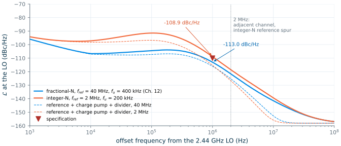
Three things get worse at once. The loop bandwidth must stay well below the reference, because the loop is sampled (Section 12.6 found it unstable above \(f_{ref}/3.4\)) and because the reference ripple must be filtered; with \(f_u = f_{ref}/10\) the loop runs at 200 kHz instead of 400 kHz. The ratio is twenty times larger, so the in-band noise of the charge pump and the divider, which reach the output multiplied by \(N\), rise by about \(10\log 20\) = 13 dB (the crystal’s contribution does not change: the reference divider divides its phase by the same factor). And the reference spur now sits at 2 MHz, on the adjacent channel, with a ripple that lasts twenty times longer per period.
The Chapter 12 script answers the question directly when we redesign its loop for \(f_{ref}\) = 2 MHz, \(N\) = 2440 and \(f_u\) = 200 kHz (Figure 14.2). The filter changes to \(R_1\) = 245 kΩ and \(C_{tot}\) = 12.7 pF. The in-band noise of reference, charge pump and divider at 100 kHz rises from −107.3 to −96.8 dBc/Hz at the LO, the total at 1 MHz from −113.0 to −108.9 dBc/Hz, which fails the −110 dBc/Hz specification, and the jitter from 451 to 1340 fs. The 1 nA of leakage that gave a −127 dBc spur at 40 MHz in Chapter 12 gives −50.5 dBc at 2 MHz. Integer-N is the wrong architecture for this radio.
A fractional-N synthesizer keeps the 40 MHz reference and lets the divider ratio have a fractional part \(\alpha\) on average [11, 21]:
Key equation · Fractional division
\[N = \frac{f_{LO}}{f_{ref}} = N_{int} + \alpha, \qquad \alpha = \frac{K}{2^B} \tag{14.1}\]
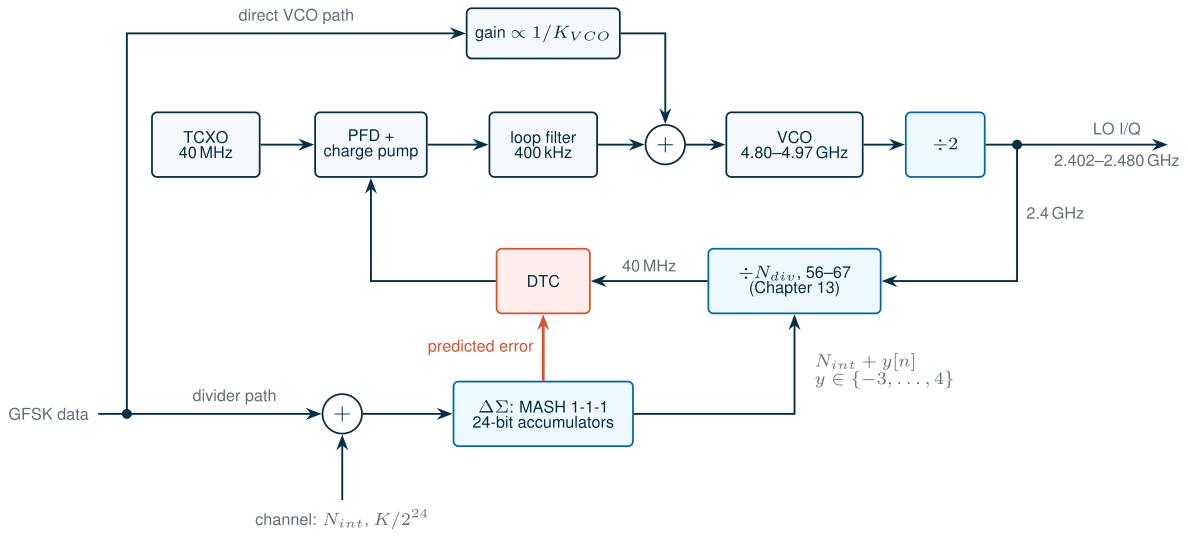
For the course radio \(N_{div}\) = 60.05–62.00, and the fraction is a multiple of 0.05. With a \(B\) = 24-bit word \(K\) the frequency resolution is \(f_{ref}/2^{24}\) = 2.38 Hz, and the largest rounding error of any BLE channel is 0.954 Hz. Figure 14.1 shows the synthesizer the rest of the chapter builds: Chapter 12’s loop, Chapter 13’s divider, a delta-sigma modulator that chooses the divider ratio every reference cycle, a digital-to-time converter that removes most of the error it leaves, and the two modulation paths of the GFSK transmitter.
14.2 Fractional division and fractional spurs
The simplest way to divide by 60.05 is to divide by 60 nineteen times and by 61 once, every 20 reference cycles. An accumulator does this for any fraction: every reference cycle it adds \(K\) to a \(B\)-bit register, and when the register overflows its carry makes the divider count one extra cycle. The average ratio is exactly Eq. (14.1) [11].
The average is right; the instantaneous phase is not. Between carries the divider’s output edge comes early by a little more each cycle, by \(\alpha\) of an LO period per reference cycle, and the extra cycle pulls it back (Figure 14.3a). The phase detector sees a sawtooth timing error one LO period high (410 ps), repeating at \(\alpha f_{ref}\). A periodic phase error is a set of tones, the fractional spurs, at
\[f_{spur} = \min(\alpha, 1 - \alpha)\,f_{ref} \tag{14.2}\]and its harmonics. For the BLE channels the fundamental falls at 2 MHz multiples: 2 MHz for the channels with \(\alpha\) = 0.05 or 0.95, exactly on the adjacent channel.
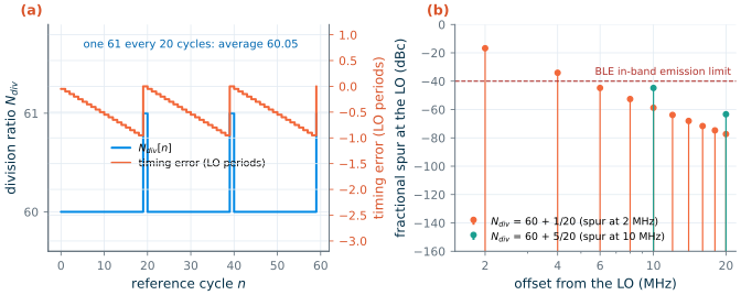
How large are they? The sawtooth’s fundamental has a peak of about 2 rad at the LO, a spur near 0 dBc before the loop (the small-angle approximation behind “dBc” is already strained there). The loop passes it with \(\lvert H(2\,\text{MHz})\rvert\) = −16.8 dB, so the 2402 MHz channel carries a spur of −16.8 dBc at 2 MHz (Figure 14.3b). Over the 38 channels that have a fraction (2440 and 2480 MHz are integer), the largest spur ranges from −57.3 dBc at best to −16.8 dBc at worst, against the −40 dBc that BLE’s in-band emission limit allows and the far lower level that the course receiver’s blocking case needs. A narrower loop would help only at the price of everything Section 14.1 was trying to avoid. The pattern itself has to go.
14.3 Delta-sigma modulators
A delta-sigma (ΔΣ) modulator chooses the sequence of integers so that its error from the wanted fraction is not periodic but noise-like, and pushed to high frequencies where the loop filter removes it. The idea came to frequency synthesis from oversampled data converters [146]. The most common form in synthesizers is the MASH (multi-stage noise shaping) modulator of Miller and Conley [147]: a cascade of \(L\) accumulators, each fed with the residue of the one before (Figure 14.4). Their carries are recombined through differentiators, \(y = c_1 + (1 - z^{-1})c_2 + (1 - z^{-1})^2c_3 + \dots\), so that the errors of all stages but the last cancel:
Key equation · MASH 1-1-…-1 of order L
\[Y(z) = \alpha + (1 - z^{-1})^L\,E(z), \qquad y[n] \in \{-(2^{L-1} - 1), \dots, 2^{L-1}\} \tag{14.3}\]

\(E\) is the last accumulator’s quantization error, close to white and uniform with variance 1/12 when the input keeps the accumulators busy. The modulator is made of accumulators only, so it is unconditionally stable. The price of a higher order is a wider output: the divider ratio \(N_{int} + y[n]\) swings over 2 values for \(L\) = 1, 4 for \(L\) = 2, 8 for \(L\) = 3 and 16 for \(L\) = 4.
The divider’s timing error is the running sum of \(y - \alpha\), which removes one differentiator. One step is one LO period, so the phase error at the LO is \(2\pi(1 - z^{-1})^{L-1}e[n]\) and its spectrum follows directly [146, 148]:
Key equation · Quantization phase noise of a MASH-L modulator
\[\mathcal{L}_{q}(f) = \frac{(2\pi)^2}{12\,f_{ref}}\left[2\sin\frac{\pi f}{f_{ref}}\right]^{2(L-1)} \tag{14.4}\]
Derivation · Eq. (14.4)
After \(n\) cycles the divider output has drifted by \(\Delta t[n] = T_{LO}\sum_{k \le n}(y[k] - \alpha)\). With Eq. (14.3), \(\sum(y - \alpha) = (1 - z^{-1})^{L-1}e\). The phase error, in radians of the LO, is \(2\pi\Delta t/T_{LO}\). The sequence \(e[n]\) is white with variance 1/12 and one sample per reference period, so its two-sided spectral density is \(1/(12f_{ref})\); the filter \((1 - z^{-1})^{L-1}\) multiplies it by \(\lvert 1 - e^{-j2\pi f/f_{ref}}\rvert^{2(L-1)} = [2\sin(\pi f/f_{ref})]^{2(L-1)}\). \(\mathcal{L}(f)\) is the two-sided phase spectrum, which gives Eq. (14.4). At the PFD, in radians of the reference, the error is \(1/N_{div}\) of this; the loop multiplies it back by \(N_{div}H\), which gives Eq. (14.5). At the VCO, twice the frequency, it is 6 dB higher, which is how the script adds it to Chapter 12’s VCO-referred contributions.
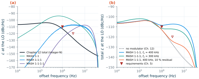
The script models the modulators bit-exactly, as cumulative sums taken modulo \(2^{24}\), with the first accumulator seeded with an odd value to break the short cycles of simple fractions. For the 2442 MHz channel (\(\alpha\) = 0.05, \(K\) = 838861) over a million reference cycles, Figure 14.5a compares the simulated phase spectrum with Eq. (14.4). The MASH 1-1-1 matches it within 0.001 dB on average from 100 kHz to 10 MHz; the MASH 1-1 within 0.07 dB on average, but its spectrum is made of closely spaced tones, because two stages are too few to whiten a simple fraction; the first-order accumulator is pure tones, at 2 MHz multiples. Before any loop filtering, the MASH 1-1-1 gives −103.0 dBc/Hz at 1 MHz and −84.1 dBc/Hz at 3 MHz: noise is rising at 40 dB per decade, and the loop has to remove it.
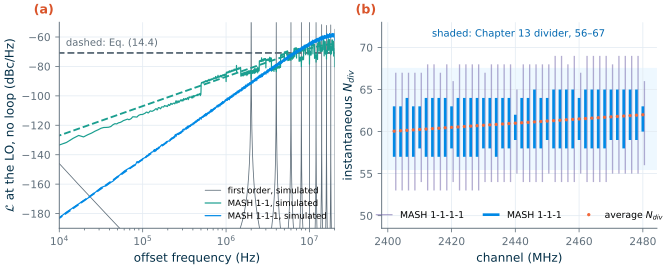
The divider sets the order. Chapter 13’s pulse-swallow divider covers \(N_{div}\) = 56–67, a range chosen for a third-order MASH with a step to spare at each end. Figure 14.5b checks it for every channel: the MASH 1-1-1 adds −3 to +4 to \(N_{int}\) as Eq. (14.3) says, and the instantaneous ratio stays within 57–65 for all 40 channels. A MASH 1-1-1-1 swings over −7 to +7 in a million cycles (Eq. 14.3 allows +8) and would need 53–69, outside the divider. The accumulated timing error of the MASH 1-1-1 spans 3.95 LO periods, 1.62 ns at 2.44 GHz, with a mean magnitude of 0.583 LO periods; both numbers return in Section 14.5.
14.4 Quantization noise in the loop
The loop treats the modulator’s phase error like any other error at the phase detector: it passes it low-pass, through the closed-loop response \(H = G/(1+G)\) of Section 12.3:
\[\mathcal{L}_{\Delta\Sigma}(f) = \lvert H(f)\rvert^2\,\mathcal{L}_{q}(f) \tag{14.5}\]The course loop’s \(\lvert H\rvert^2\) falls at 20 dB per decade above \(f_u\) (its zero is at 108 kHz and its poles at 1.75 and 11.6 MHz), then at 40 and 60 dB per decade. Against noise rising at 40 dB per decade, the product of a MASH 1-1-1 and the course loop climbs for another decade, peaks at −107.3 dBc/Hz near 3.31 MHz, and falls only beyond the third pole. A modulator of order \(L\) needs a loop whose response falls faster than \(20(L-1)\) dB per decade, or its noise never comes down [148, 11].
Worked example 14.1 · The MASH 1-1-1 at 1 MHz, by hand
Eq. (14.4) at 1 MHz with \(f_{ref}\) = 40 MHz: \((2\pi)^2/(12 \times 40\,\text{MHz})\) is −70.85 dBc/Hz, and \([2\sin(\pi/40)]^4\) adds −32.2 dB, which gives −103.0 dBc/Hz at the LO before the loop. The course loop has \(\lvert H(1\,\text{MHz})\rvert^2\) = −7.5 dB (1 MHz is only 2.5 \(f_u\)), so the modulator contributes −110.5 dBc/Hz, more than Chapter 12’s own total of −113.0 dBc/Hz. Their sum is −108.6 dBc/Hz: the specification fails by 1.4 dB, before the charge pump’s longer on-time is even counted.
Figure 14.6a adds the three MASH orders to Chapter 12’s integer-N total with contributions() and to_lo(), and Table 14.1 lists the result. The script also lengthens the charge pump’s on-time: the modulator’s timing error keeps one current source on for 239 ps per period on average, which raises the charge pump’s effective duty from 2.0 % to 2.48 % (Section 12.3’s duty-cycle scaling, with one source counted at half the noise of two).
Table 14.1. Choosing the modulator for the course loop (fu = 400 kHz unless noted, Chapter 11's simulated VCO, LO-referred, 2442 MHz channel). Jitter integrated from 10 kHz to 10 MHz. Requirements: −110 dBc/Hz at 1 MHz and −119.9 dBc/Hz at 3 MHz (Chapter 5).
| Modulator | In the 56–67 range? | 1 MHz | 3 MHz | Jitter |
|---|---|---|---|---|
| none (integer-N, Chapter 12) | — | −113.0 | −127.1 | 451 fs |
| MASH 1-1 | yes | −94.4 | −100.7 | 2690 fs |
| MASH 1-1-1 | yes (57–65) | −108.5 | −107.3 | 1170 fs |
| MASH 1-1-1-1 | no (53–69) | −112.4 | −113.7 | 1010 fs |
| MASH 1-1-1, fu = 300 kHz | yes | −111.6 | −112.2 | 751 fs |
| MASH 1-1-1 with 10 % residual (Section 14.5) | yes | −112.9 | −124.2 | 465 fs |
Phase noise in dBc/Hz.
No modulator alone meets both requirements. The MASH 1-1 is hopeless. The MASH 1-1-1 fails at 1 MHz by 1.5 dB and misses the 3 MHz requirement, which Chapter 5 set for the course receiver’s blocker case, by 12.6 dB. The MASH 1-1-1-1 meets 1 MHz but needs a divider range we do not have, and still fails at 3 MHz. Narrowing the loop to 300 kHz rescues the 1 MHz point with 1.6 dB to spare, but not 3 MHz; it also raises the jitter to 751 fs and the filter capacitance from 63.5 to 113 pF, because the in-band noise now reaches further out and \(C_{tot}\) grows as \(1/f_u^2\). Moving the third pole down (Chapter 12’s Try-it) attenuates the hump beyond 3 MHz but does nothing at 1 MHz, where \(H\) is set by the loop gain itself.
The remaining lever is to stop the error from reaching the phase detector at all. The modulator’s timing error is not random to the designer: the digital logic knows \(\sum(y - \alpha)\) exactly, one cycle ahead. If a circuit removes all but a fraction \(\delta\) of it, Eq. (14.5) gains a factor \(\delta^2\). With \(\delta\) = 10 %, an assumed gain accuracy that a background calibration reaches comfortably, the MASH 1-1-1 contributes −130.5 dBc/Hz at 1 MHz and the synthesizer meets both points (Figure 14.6b). Section 14.6 replaces the assumption with a model of the DTC and its calibration, and the course budget uses that model. The course synthesizer uses a MASH 1-1-1 with quantization-error cancellation. The next section says how, and why the cancellation is worth having for a second reason.
14.5 Nonlinearity and spur cancellation
So far the charge pump has been linear: a timing error \(\Delta t\) delivers a charge \(I_{CP}\Delta t\), whatever its sign. A real charge pump’s UP and DN currents differ. Chapter 12’s SG13G2 charge pump mismatches by 0.77 % at mid-rail and by up to 4.0 % over 0.3–0.9 V. A positive error is then integrated by the UP source and a negative one by the DN source, and the charge per period becomes piecewise-linear:
\[\frac{Q}{I_{CP}} = \Delta t\left(1 \pm \frac{\varepsilon}{2}\right) + \varepsilon\,t_{rst} \qquad (+\ \text{for}\ \Delta t > 0) \tag{14.6}\]In an integer-N loop the error is tiny and of one sign, and the kink does no harm. In a fractional-N loop the modulator’s error swings over 1.62 ns, through zero, every few cycles. A nonlinearity applied to shaped noise mixes its high-frequency components down: the noise that the modulator so carefully pushed above 1 MHz folds back into the loop band, and the periodicity hidden in a simple fraction reappears as fractional spurs [150, 149].
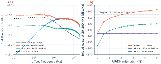
The script estimates the effect behaviourally. It applies Eq. (14.6) to the bit-exact MASH 1-1-1 timing error of the 2442 MHz channel, lets the loop settle to the static offset that makes the average charge zero (−24.8 ps for 4 % mismatch), and takes the spectrum of the charge sequence as an equivalent phase error, which the loop filters with \(H\). The VCO’s own phase moves far less than the 1.62 ns of the modulator, so it is ignored inside the nonlinearity. Figure 14.7 is the result. With 4.0 % mismatch, the folded noise is a flat floor of −99.2 dBc/Hz from 20 to 200 kHz, above Chapter 12’s whole in-band total (−104.5 dBc/Hz), which it would raise to −98.1 dBc/Hz; a fractional spur appears at 2 MHz at −67.0 dBc. At the mid-rail mismatch of 0.77 % the floor is −113.5 dBc/Hz, still only 9 dB below the in-band total. Every percent of mismatch counts.
There are three cures, all in use [11, 21]:
- An offset current. A small constant current into the loop filter moves the lock point until the timing error has one sign; the kink is never crossed and the folding disappears (Figure 14.7b, flat at −135.6 dBc/Hz). The offset must cover the whole swing, 906 ps here, so one source now conducts for most of a nanosecond every period: the duty rises to 3.81 % and the charge pump’s in-band noise from −110.5 to −107.6 dBc/Hz. It also brings back a reference spur, now from a deliberate leak.
- Quantization-error cancellation. Because the error is known, it can be cancelled. Pamarti, Jansson and Galton subtracted it as a charge, with a DAC driven from the modulator, in a 2.4 GHz synthesizer modulated at 1 Mb/s, exactly the course’s application [149]. A digital-to-time converter (DTC) does it in the time domain instead: it delays the divider’s output edge by the predicted error, so the phase detector sees only the residue \(\delta\sum(y - \alpha)\). That shrinks everything at once: the quantization noise by \(\delta^2\) (Section 14.4), the swing that the kink folds (−120.8 dBc/Hz at 4 % for \(\delta\) = 10 %) and the on-time (duty 2.05 %). The DTC must span 1.62 ns, and its own noise, nonlinearity and gain calibration become the new limits; Section 14.6 models them.
- Dithering. Adding a pseudo-random least-significant bit to \(K\), or seeding the accumulators as the script does, breaks the short cycles that turn folded noise into spurs, at the cost of a slightly higher floor [147, 149].
Common pitfall · Verifying a fractional-N loop with an ideal charge pump
A linear phase-domain model with Eq. (14.5) predicts the quantization noise perfectly and says nothing about folding: the in-band floor of Figure 14.7 does not exist in it. Always run the modulator’s actual sequence through a model of the phase detector with the mismatch, timing skew and dead zone of the real charge pump, and do it at the fractions near zero, one half and one, where the sequences are the most regular.
14.6 The course fractional-N synthesizer
Channel words
Table 14.2 gives the words for a few channels; the script lists all 40. Each channel needs only \(N_{int}\) = 60, 61 or 62 and a fraction that is a multiple of 0.05. Two channels, 2440 and 2480 MHz, are integer: the modulator is idle there and adds no noise or spurs, which a design either accepts or avoids by offsetting the integer part and using \(\alpha\) = 1.
Table 14.2. Channel words of the course synthesizer (fref = 40 MHz, 24-bit fraction). Over all 40 channels the MASH 1-1-1 keeps the instantaneous ratio within 57–65 (Figure 14.5b).
| LO (MHz) | Ndiv | Nint | α | K | LO error |
|---|---|---|---|---|---|
| 2402 | 60.05 | 60 | 0.05 | 838861 | 0.477 Hz |
| 2404 | 60.1 | 60 | 0.1 | 1677722 | 0.954 Hz |
| 2440 | 61.0 | 61 | 0 | 0 | 0 |
| 2442 | 61.05 | 61 | 0.05 | 838861 | 0.477 Hz |
| 2460 | 61.5 | 61 | 0.5 | 8388608 | 0 |
| 2478 | 61.95 | 61 | 0.95 | 15938355 | −0.477 Hz |
| 2480 | 62.0 | 62 | 0 | 0 | 0 |
Two-point GFSK modulation
The transmitter of Chapter 5 sends GFSK by steering the synthesizer itself: BLE’s modulation index of 0.5 needs a deviation of ±250 kHz at the LO. Through the divider this is simply a change of the fraction, ±0.00625 in \(N_{div}\) or ±104858 in \(K\), which the modulator applies within one reference cycle. But the loop passes the divider path through \(H\), and the 1 Mb/s data has most of its energy around 500 kHz, beyond the 400 kHz bandwidth: \(\lvert H\rvert\) is 1.19 at 250 kHz (the loop’s peaking) and 0.864 at 500 kHz, enough to distort the frequency pulses. Two-point modulation adds the same data directly to the VCO’s tuning input, where the loop passes it through \(1 - H\) [11, 21]. With \(K_{VCO}\) = 131 MHz/V, ±500 kHz at the VCO is ±3.81 mV. If the direct path’s gain is off by \(\gamma\),
\[\frac{\Delta f_{out}}{\Delta f_{cmd}} = H + (1 + \gamma)(1 - H) = 1 + \gamma\,(1 - H) \tag{14.7}\]so the response is flat only if the two gains match. Even after band calibration \(K_{VCO}\) ranges over 103–167 MHz/V (Section 11.8), up to 27.3 % from its design value; uncalibrated, that is a deviation error of up to 30.3 % at 500 kHz, where \(\lvert 1 - H\rvert\) = 1.11. The direct path’s gain must therefore be calibrated against the divider path, which is exact. The alternatives are a loop wide enough to pass the data, as in Pamarti’s 1 Mb/s in-loop modulation with quantization-noise cancellation [149], or digital pre-emphasis of the divider command by the inverse of \(H\) [78]. Near an integer channel the data pushes \(\alpha\) below zero; the channel word then simply moves to \(N_{int} - 1\), and the instantaneous ratio still stays within the divider’s range.
The DTC, modelled
Section 14.4 rested on one assumption: that the DTC leaves 10 % of the modulator’s timing error. Chapter 19 shows how much depends on it: the 3 MHz requirement holds only for residuals below 21 %. This subsection replaces the assumption with a behavioural model of the DTC, its impairments and its calibration, and the completed budget at the end of the section uses the model.
What the DTC must do. Every reference cycle the modulator’s logic knows the timing error of the next divider edge, \(x[n] = \sum(y - \alpha)\) in LO periods. For the MASH 1-1-1 this is \(e[n] - 2e[n-1] + e[n-2]\), which lies within ±2 LO periods. The DTC delays the edge by \((2 - x[n])\,T_{LO}\), so the phase detector sees a constant. Its range must therefore be four LO periods at the lowest channel: 1.67 ns at 2402 MHz (the simulated MASH 1-1-1 uses 1.62 ns of it).
The assumed DTC. We assume the most common kind, a variable-slope DTC: a gate charges a digitally switched capacitor bank, and the next gate fires when the ramp crosses its threshold [151, 176]. A delay of 2.5 ns in a 1.2 V, 130 nm process also needs a coarse delay line, so we let the two most significant bits select one of four line segments and the capacitor bank interpolate within them. With 11 bits and a nominal step \(\Delta\) = 1.2 ps the full scale is 2.46 ns, which still covers 1.67 ns when the DTC is up to 32 % slower than nominal. Four impairments, all assumed rather than simulated at transistor level:
- Gain error. The delay per code is \(g\Delta\), with \(g\) set by process, supply and temperature. We take a die 30 % slow, \(g\) = 0.7, Chapter 19’s starting point.
- Resolution. The code is rounded to whole steps. With \(g\Delta\) = 0.84 ps the rounding error is 0.24 ps rms, if it is white.
- Integral nonlinearity (INL). A variable-slope stage is not linear in its code: the slope of the ramp changes with the load, and the next gate’s delay changes with the slope [151]. We take a smooth bow, 10 ps at mid-scale (0.4 % of the full scale), plus offset steps at the three boundaries between the coarse segments, drawn with σ = 2 ps (here +1.39, −1.96 and −3.14 ps).
- Jitter. 0.5 ps rms per edge, independent of the code. About 60 gate delays make up 2.5 ns, and \(\sqrt{60}\) times Chapter 13’s 40.5 fs per gate is 0.31 ps; the slow ramp of the interpolator adds the rest.
The delay of edge \(n\), and the code that sets it, are then
\[\tau[n] = g\,\Delta\,c[n] + \mathrm{INL}(c[n]) + \sigma_j\,w[n], \qquad c[n] = \mathrm{round}\!\left[\hat g\,(2 - x[n])\,\frac{T_{LO}}{\Delta}\right] \tag{14.8}\]where \(\hat g\) is the digital gain (ideally \(1/g\)) and \(w[n]\) is white noise of unit variance. The phase detector sees \(x[n]\,T_{LO} + \tau[n]\). The script passes this residue through the loop exactly as Section 14.4 passed \(\delta\,x\), on the bit-exact MASH 1-1-1 sequence of the 2442 MHz channel, and adds it to Chapter 12’s sources with budget_dtc().
White timing noise. Jitter, and roughly the rounding error, add a white timing error \(\sigma_t\) to every edge at the phase detector. Like the divider’s jitter in Chapter 12, the loop passes it to the LO multiplied by the division ratio:
Key equation · White timing noise at the phase detector
\[\mathcal{L}(f) = \lvert H(f)\rvert^2\,\frac{(2\pi f_{LO}\,\sigma_t)^2}{f_{ref}}, \qquad \sigma_t^2 = \sigma_j^2 + \frac{(g\Delta)^2}{12} \tag{14.9}\]
Worked example 14.2 · The DTC’s jitter at 1 MHz, by hand
With \(\sigma_j\) = 0.5 ps at 2.442 GHz, \(2\pi f_{LO}\sigma_j\) = 7.67 mrad. Squared and divided by 40 MHz, this is −118.3 dBc/Hz in band (1 ps would give −112.3 dBc/Hz, as Chapter 13 found for the divider). At 1 MHz the loop’s \(\lvert H\rvert^2\) of −7.5 dB brings it to −125.8 dBc/Hz, which raises Chapter 12’s −113.0 dBc/Hz to −112.8. The requirement of −110 dBc/Hz leaves room for −113.0 dBc/Hz more at 1 MHz, so the DTC’s white timing noise may reach about 2.2 ps rms before the 1 MHz point fails.
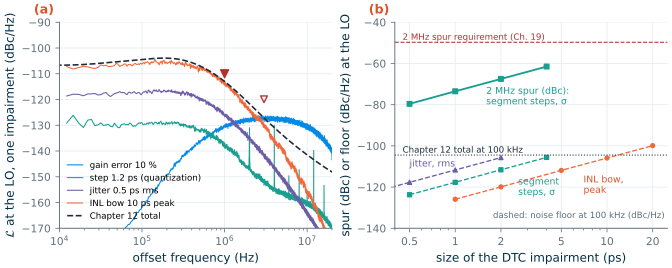
Figure 14.8a shows what each impairment leaves at the LO on its own, and Table 14.3 lists the totals. A gain error is exactly the \(\delta\) of Section 14.4: its residue is a scaled copy of the modulator’s shaped error, rising at 40 dB per decade, and 30 % of it gives −117.4 dBc/Hz at 3 MHz. Jitter is flat in band, as Eq. (14.9) says; the sweep agrees with the 2.2 ps limit (2 ps gives −110.4 dBc/Hz at 1 MHz). Rounding with a 1.2 ps step stays 5 dB below Eq. (14.9)’s white estimate, at −129.3 dBc/Hz in band, because the codes take few distinct values: at \(\alpha\) = 0.05 the fractional part of \(x\) repeats every 20 cycles. For the same reason part of its power appears as lines near multiples of 2 MHz, from −101 dBc for a 0.6 ps step to −84.5 dBc for 2.4 and 4.8 ps; dithering the DTC’s last bit would spread them.
The INL is the impairment that matters. It is a nonlinearity in the path of the shaped error, like the charge-pump mismatch of Section 14.5, and it folds the modulator’s high-frequency noise into the band. A 10 ps bow alone gives a floor of −105.9 dBc/Hz at 100 kHz and −110.3 dBc/Hz at 1 MHz in total, only 0.3 dB inside the requirement. A smooth bow folds into noise, with no line above it at 2442 MHz. The segment steps are kinks, like the charge pump’s, and they make tones: steps of σ = 2 ps give a 2 MHz spur of −67.5 dBc and a floor of −111.6 dBc/Hz (Figure 14.8b). Every doubling of the bow, the steps or the jitter costs 6 dB.
Calibration. Two sign-sign LMS loops in the modulator’s logic fix what can be fixed. Both use the sign of the phase error at each reference edge, from a flip-flop that compares the DTC’s output with the reference (a bang-bang detector beside the PFD). The gain loop steps \(\hat g\) by \(\mu\) = 4 × 10⁻⁴ in the direction given by that sign times the sign of \(x[n]\), as in Chapter 19. The INL loop, in the spirit of Levantino et al. [176], adds a piecewise-linear pre-distortion with 16 segments to the code and steps its 15 interior nodes by 0.02 ps, each weighted by where the code lies between its two nodes; its end nodes stay at zero, so it does not fight the gain loop. As in Chapter 19, 0.5 ps of random timing noise at the detector stands for the loop’s own phase noise.
Figure 14.9a shows the two loops at work. The gain falls from 30 % below 10 % in 19.8 µs and below 2 % in 28.9 µs, then wanders by 0.34 % rms; Chapter 19’s 18 µs had no INL, jitter or rounding to contend with. The gain loop alone leaves the nonlinearity: 2.2 ps rms once the codes span the whole range. The INL loop brings it below 1 ps in 224 µs and to 0.52 ps rms, which includes the 0.24 ps of rounding. The piecewise-linear correction cannot follow a step within a segment, so a 2 MHz spur of −81.5 dBc remains.
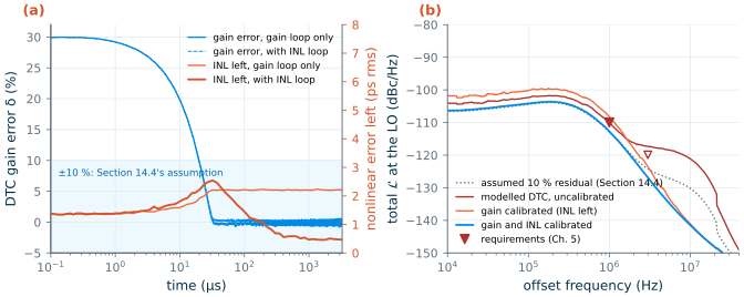
Table 14.3. DTC impairments against results (2442 MHz channel, Chapter 11's simulated VCO, totals at the LO including Chapter 12's sources and the charge pump's on-time). Single impairments use an otherwise ideal DTC. δeff: the gain error that would leave the same DTC contribution at 3 MHz. Spur: the largest line near multiples of 2 MHz through the loop, "none" when no line stands 15 dB above the noise.
| DTC | 100 kHz | 1 MHz | 3 MHz | Jitter | Spur (dBc) | δeff |
|---|---|---|---|---|---|---|
| assumed 10 % residual (Section 14.4) | −104.4 | −112.9 | −124.3 | 465 fs | none | 9.9 % |
| gain error 30 % | −104.4 | −112.3 | −117.4 | 557 fs | none | 29.8 % |
| gain error 2 % | −104.5 | −113.0 | −127.0 | 452 fs | none | 2.0 % |
| step 1.2 ps (11 bits) | −104.5 | −113.0 | −127.1 | 452 fs | −95.1 at 4 MHz | 0.6 % |
| step 4.8 ps (9 bits) | −104.0 | −112.5 | −126.7 | 481 fs | −84.5 at 6 MHz | 3.4 % |
| jitter 0.5 ps rms | −104.3 | −112.8 | −127.0 | 463 fs | none | 1.9 % |
| jitter 2 ps rms | −102.0 | −110.4 | −125.2 | 612 fs | none | 7.7 % |
| INL bow 10 ps | −102.1 | −110.3 | −125.3 | 596 fs | none | 7.5 % |
| segment steps σ = 2 ps | −103.7 | −112.1 | −126.5 | 495 fs | −67.5 at 2 MHz | 4.0 % |
| course DTC, uncalibrated | −102.3 | −110.1 | −117.4 | 663 fs | −68.4 at 2 MHz | 29.8 % |
| gain calibrated (LMS) | −100.2 | −108.2 | −123.6 | 748 fs | −67.6 at 2 MHz | 11.6 % |
| gain and INL calibrated (the course DTC, Table 14.4) | −104.2 | −112.7 | −126.9 | 467 fs | −81.5 at 2 MHz | 2.4 % |
| the same, with 4 % pump mismatch | −104.2 | −112.7 | −126.9 | 467 fs | −81.7 at 2 MHz | 2.4 % |
| Requirements (Chapters 5 and 19) | −110 | −119.9 | −49.7 |
Phase noise in dBc/Hz. The course DTC has all four impairments: g = 0.7, a 1.2 ps step, 0.5 ps of jitter, a 10 ps bow and the segment steps above.
Uncalibrated, the course DTC fails the 3 MHz point (−117.4 dBc/Hz) and keeps only 0.1 dB at 1 MHz (−110.1 dBc/Hz). With only its gain calibrated, 3 MHz passes but 1 MHz gets worse and fails, −108.2 dBc/Hz, for the reason the pitfall below explains. With both loops the synthesizer reaches −112.7 dBc/Hz at 1 MHz and −126.9 dBc/Hz at 3 MHz: margins of 2.7 and 7.0 dB. Chapter 12’s 4 % pump mismatch now changes nothing visible, because the residue is too small to fold. The 2 MHz spur of −81.5 dBc is 31.8 dB inside the −49.7 dBc that Chapter 19 allows for a −50 dBm interferer 2 MHz away, and 41.5 dB inside BLE’s −40 dBc.
The effective residual is not one number. The calibrated DTC’s residue is not a scaled copy of the modulator’s error. At 3 MHz, where Chapter 19’s 21 % limit applies, it is worth δ = 2.4 %, a quarter of the assumed 10 %, and the 3 MHz total improves from −124.3 to −126.9 dBc/Hz. In band it is a white floor that the assumption did not have: −115.6 dBc/Hz at 100 kHz from the jitter, the INL left over and the rounding, which costs 0.2 dB at 1 MHz (−112.7 instead of −112.9 dBc/Hz) and 2 fs of jitter. The 10 % of Section 14.4 was therefore pessimistic at 3 MHz and slightly optimistic at 1 MHz. Since the model captures both effects, and the assumption neither, the course budget uses the modelled DTC from here on: the calibrated case, provided its INL is calibrated and its jitter stays well below 2.2 ps.
Common pitfall · Calibrating only the DTC’s gain
A gain loop converges in microseconds and makes the cancellation look finished. But a DTC 30 % slow needs codes 43 % larger once its gain is corrected, so the calibrated DTC uses its whole range, and with it the whole of its INL bow: the nonlinear error grows from 1.4 to 2.2 ps rms, and the 1 MHz point falls from −110.1 to −108.2 dBc/Hz. Check the residue’s spectrum in band, not just the gain, and calibrate the INL with the same machinery.
The completed budget
Table 14.4 completes Chapter 12’s Table 12.2 for the fractional-N synthesizer. Its ΔΣ row is no longer an assumed residual: it is the modelled DTC of the previous subsection with its gain and INL calibrated, run on the bit-exact MASH 1-1-1 sequence of the 2442 MHz channel, so it carries the quantization noise that the DTC leaves, the DTC’s own jitter and rounding, and what remains of its INL. The charge pump has the on-time that this residue leaves (duty 2.0 %, as in integer-N), and the VCO is the one Chapter 11 simulated. The course synthesizer reaches −112.7 dBc/Hz at 1 MHz, 2.7 dB inside the specification, and −126.9 dBc/Hz at 3 MHz, 7.0 dB inside the blocker requirement, with 467 fs of jitter (0.410° rms at the LO) against 451 fs for the integer-N loop of Chapter 12. The ΔΣ row, 123 fs, now sits below every other significant source at every offset: its in-band floor (−115.6 dBc/Hz at 100 kHz) is 5 dB under the reference and the charge pump, and at 3 MHz, where a 10 % residual would make it the largest source, it is 7.6 dB under the VCO.
Table 14.4. Phase-noise budget of the course fractional-N synthesizer at the 2.44 GHz LO (fu = 400 kHz, ICP = 100 µA, KVCO = 131 MHz/V, third-order filter, Chapter 11's simulated VCO, MASH 1-1-1 with the modelled DTC, gain and INL calibrated). Each row is one source's contribution through the closed loop; jitter from 10 kHz to 10 MHz.
| Source (model) | 100 kHz | 1 MHz | 3 MHz | 10 MHz | Jitter |
|---|---|---|---|---|---|
| TCXO, 40 MHz (Chapter 12) | −110.1 | −118.8 | −134.6 | −157.0 | 236 fs |
| Charge pump, duty 2.0 % | −110.5 | −119.2 | −135.0 | −157.4 | 223 fs |
| R1 = 24.5 kΩ | −115.2 | −120.6 | −136.3 | −158.7 | 171 fs |
| R3 = 19.0 kΩ | −116.0 | −120.9 | −133.9 | −148.3 | 162 fs |
| Divider, retimed (Chapter 12) | −136.0 | −144.6 | −160.4 | −182.8 | 11.9 fs |
| Divide-by-two floor (Chapter 13) | −158.1 | −158.1 | −158.1 | −158.1 | 3.63 fs |
| VCO (Chapter 11, simulated) | −109.4 | −120.9 | −132.1 | −143.1 | 206 fs |
| ΔΣ quantization noise with the modelled DTC (gain and INL calibrated) | −115.6 | −124.4 | −139.7 | −162.2 | 123 fs |
| Total | −104.2 | −112.7 | −126.9 | −141.5 | 467 fs |
| Requirements (Chapter 5) | −110 | −119.9 |
Phase noise in dBc/Hz. Folding by charge-pump mismatch changes nothing visible: with Chapter 12’s worst-case 4 % mismatch the totals are the same (Table 14.3, last row), because the DTC’s residue is too small to fold.
Sensitivity. Two inputs of this budget used to be ranges. With Chapter 11’s first VCO estimate (noise factor F = 2–5, 1/f³ corner assumed at 1 MHz) in place of its simulation, the totals would be −112.6 to −111.7 dBc/Hz at 1 MHz and −127.2 to −125.8 dBc/Hz at 3 MHz, with 476–551 fs of jitter. With Section 14.4’s 10 % residual in place of the modelled DTC, they would be −112.9 and −124.2 dBc/Hz (465 fs). Neither changes a conclusion: the VCO matters most at 1 MHz, the DTC at 3 MHz.
What this means for your design
In a fractional-N synthesizer the modulator, the divider and the loop filter are one design. The divider’s range caps the modulator’s order (here at three); the order and the reference set how fast the quantization noise rises; and the loop must fall faster still, at an offset that the receiver’s blocking requirement may care about more than the headline 1 MHz point. When the numbers do not close, as they did not here by 1.5 dB at 1 MHz and 12.6 dB at 3 MHz, cancelling the known error is cheaper than narrowing the loop, and it also removes most of the charge pump’s nonlinearity.
A taped-out comparison
The open-source SG13G2 fractional-N PLL of Thiriloganathan et al. [106, 207] made the opposite set of choices. Its VCO runs at 2.4 GHz with a 10 MHz reference, and a first-order delta-sigma modulator dithers the division ratio between 240 and 248, a step of 8 VCO periods (3.33 ns) because a fixed divide-by-4 precedes its dual-modulus stage (Chapter 13). Section 14.2 describes what such a modulator produces: a sawtooth timing error and spurs at multiples of the fractional offset, here from 10 MHz, not shaped away from the carrier. The step alone makes that error 18.2 dB larger than a step of one LO period (410 ps) would. In exchange the whole divider and modulator are synthesized logic, which an open-source flow lays out cleanly. Their reported spur and phase noise (Chapter 12) should be read in that light, not as a statement about the course design, whose numbers are pre-layout estimates.
Try it · The fractional-N script
Every number in this chapter comes from
tools/figs/ch14_fractional_n.py, which imports Chapter 12’s loop model;python3 tools/figs/ch14_fractional_n.pyredraws everything in under a minute. Four experiments: (1) setDELTAto 0.2 and to 0.05 and rerunnoise: how good must the cancellation be for the 3 MHz requirement alone? (2) ChangeFLOto2460e6(α = 0.5) and rerunnonlin: where do the fractional spurs of the 4 % mismatch case move, and how large are they? (3) Callmash()withseed=0for the MASH 1-1 inpart_dsmand look at its spectrum for α = 0.05: why do designers dither the least-significant bit? (4) In theDTCsettings abovepart_dtc, setseg_sigma_psto 4 and thenpwlto 4, and rerundtc course: which fails first after calibration, the 1 MHz margin or the spur budget? (budget_design()rebuilds the course budget from the calibrated DTC; passFv=5to see Chapter 11’s earlier VCO estimate instead of its simulation.)
- Integer-N steps in units of its reference. For 2 MHz channels the course loop would need a 2 MHz reference, a 200 kHz bandwidth and a ratio of 2440, and would miss its specification (−108.9 dBc/Hz at 1 MHz) with a reference spur on the adjacent channel.
- A first-order accumulator gives the right average ratio but a sawtooth phase error; its fractional spurs reach −16.8 dBc at 2 MHz through the course loop.
- A MASH-L modulator shapes the quantization error by (1 − z−1)L; the phase noise rises at 20(L − 1) dB per decade (Eq. 14.4), and the output range doubles with each order. Chapter 13’s 56–67 divider admits a MASH 1-1-1 (57–65 over all channels) but not a fourth order.
- Through the 400 kHz course loop, a MASH 1-1-1 alone gives −108.5 dBc/Hz at 1 MHz and −107.3 dBc/Hz at 3 MHz; cancelling its known timing error to a 10 % residual (DTC) restores −112.9 dBc/Hz and −124.2 dBc/Hz.
- UP/DN mismatch folds shaped noise into the band: 4 % gives a −99.2 dBc/Hz floor. An offset current removes the folding at the cost of charge-pump noise; cancellation removes most of it for free.
- The DTC must span four LO periods (1.67 ns). Its gain error acts like the residual δ; its jitter and rounding add a white floor (Eq. 14.9, 2.2 ps rms at most for the 1 MHz point); its INL folds the shaped noise into the band (a 10 ps bow alone leaves only 0.3 dB at 1 MHz), and its segment steps make fractional spurs (−67.5 dBc at 2 MHz for σ = 2 ps).
- Sign-sign LMS loops calibrate the gain (30 % to below 2 % in 29 µs) and a 16-segment INL pre-distortion (0.52 ps rms left): an effective residual of 2.4 % at 3 MHz instead of the assumed 10 %, plus an in-band floor the assumption did not have. Calibrating the gain alone makes the 1 MHz point worse.
- The course budget uses this modelled DTC and Chapter 11’s simulated VCO: −112.7 dBc/Hz at 1 MHz and −126.9 dBc/Hz at 3 MHz from the LO (2.7 and 7.0 dB of margin), 467 fs of jitter and a −81.5 dBc spur at 2 MHz. The earlier VCO bracket would give −111.7 to −112.6 dBc/Hz at 1 MHz, the 10 % residual −124.2 dBc/Hz at 3 MHz.
- GFSK is applied at two points, the divider (±104858 in the 24-bit word) and the VCO (±5.16 mV), whose gains must be matched by calibration.
Further reading
- T. A. D. Riley, M. A. Copeland and T. A. Kwasniewski [146] brought delta-sigma modulation to fractional-N synthesis; B. Miller and R. J. Conley [147] introduced the multiple-accumulator (MASH) divider.
- M. H. Perrott, M. D. Trott and C. G. Sodini [148]: the phase-domain model of a ΔΣ fractional-N synthesizer used in Section 14.4, with the sampling and divider effects it leaves out of Eq. (14.4).
- S. Pamarti, L. Jansson and I. Galton [149]: quantization-noise cancellation and 1 Mb/s in-loop modulation at 2.4 GHz; H. Arora et al. [150] for noise folding by charge-pump mismatch.
- B. Razavi, Design of CMOS Phase-Locked Loops [11], and A. L. Lacaita, S. Levantino and C. Samori [21]: fractional-N architectures, modulators, spurs and their cures in textbook form; S. Palermo’s ECEN 620 notes [2] cover the same ground in lecture form.
- S. Levantino, G. Marzin and C. Samori [176]: how a DTC’s nonlinearity creates fractional spurs, and an adaptive pre-distortion that removes them; J. Z. Ru et al. [151]: why a variable-slope DTC is nonlinear, and constant-slope charging as the cure.