Lab 6
The VCO and the PLL Loop
Part A runs Chapter 11's LC VCO in ngspice: its oscillation frequency, amplitude and current, its tuning range over the capacitor bank and the varactor, and the Q of its tank element by element. Part B closes the loop of Chapter 12 around it in python-control, from the loop filter's component values to the margins, the step response and the phase-noise budget at the LO.
- Simulate an LC oscillator from start-up to steady state and measure its frequency, amplitude, supply current and tuning gain from transients.
- Split a tank’s losses into its elements with small-signal analyses and add them with Eq. (11.4).
- Build a charge-pump PLL’s loop gain from component values as python-control transfer functions, and read its crossover, phase margin, closed-loop peaking and step response.
- Shape every noise source of the synthesizer through the loop, refer the result to the LO and integrate the jitter.
- Check both parts against Chapters 11 and 12, and say which numbers depend on which.
Contents
| Lab 6 at a glance | |
|---|---|
| Goal | Part A: the course VCO’s frequency, amplitude, tuning and tank Q from your own ngspice runs. Part B: the course PLL’s margins, closed-loop behaviour and phase-noise budget from python-control. |
| Chapters | Chapter 11 (Sections 11.2, 11.3, 11.5 and 11.8, Table 11.2); Chapter 12 (Sections 12.2–12.4 and 12.7, Worked example 12.1, Table 12.2) |
| Time | 2 × 3 hours, one session per part |
| Files | tools/labs/lab6/: vco_lab.py (Part A), pll_lab.py (Part B); they import tools/figs/_ch11_vco.py, tools/figs/_ch07_inductor.py and tools/figs/ch12_pll_noise.py, and read ch11_numbers.json, ch12_numbers.json and ch13_numbers.json in tools/figs/ |
| Run time | Part A: tune about 50 s, tank under a second; Part B: about 4 s in all |
Hand calculation
Part A. The course VCO (Figure 11.3) resonates Chapter 7’s L3 spiral, 1.98 nH, with a differential tank capacitance of 537 fF and draws a tail current of 0.6 mA.
- Frequency. Compute \(f_0 = 1/(2\pi\sqrt{LC})\).
- Tank Q. At bank code 8 the elements are: the spiral, Q = 17.8; the bank, 81.0 fF with Q = 21.6; the varactor, 76.1 fF with Q = 98.3; the fixed MIM pair, 276 fF with Q = 394; the divider input, 7.6 fF with Q = 12.2. Add them with Eq. (11.4) and give \(Q_{tank}\) and \(R_p = Q_{tank}/(\omega_0C)\).
- Amplitude. Evaluate Eq. (11.5) for the complementary pair, \(V_A \approx (4/\pi)IR_p\).
- Tuning gain. The varactor’s steepest small-signal slope is 39.7 fF/V (Worked example 11.2). Evaluate Eq. (11.7) for the peak \(K_{VCO}\).
Part B. The loop has \(f_{ref}\) = 40 MHz, \(N\) = 122, \(I_{CP}\) = 100 µA and \(K_{VCO}\) = 131 MHz/V, the centre of the 103–167 MHz/V that the loop sees after the band calibration of Section 11.8, designed for \(f_u\) = 400 kHz and PM = 60°.
- Filter shape. Eq. (12.4) gives \(b = \tan\left[(\mathrm{PM} + 90°)/2\right]\), a zero at \(f_u/b\) and a combined pole near \(bf_u\). Evaluate them, and the sibling course’s estimate \(R_1 \approx N\omega_u/(I_{CP}K_{VCO})\).
- In-band reference noise. The TCXO’s floor is −147 dBc/Hz at 40 MHz. What is it at the 4.88 GHz VCO inside the loop bandwidth, and at the 2.44 GHz LO?
Steps, Part A: the VCO
Work in tools/labs/lab6. Inside the container run the commands as shown; from your own computer, put ../common/iic.sh in front of each (Lab 0).
-
Transients.
cd /foss/designs/rfic-design/tools/labs/lab6
python3 vco_lab.py tune               # from your computer: ../common/iic.sh python3 vco_lab.py tune
The script writes
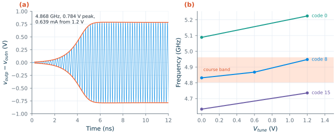
out/vco_tune.cirand runsngspice -bon it. The circuit lines come fromvco_lines()oftools/figs/_ch11_vco.py: the complementary pair (M1–M4 as eight RF instances each), the tail mirror with its RC filter, the L3 spiral as its EM-fitted π model, the varactorXV, the four bank bits (XB…, the switchesXS…and their gate and bias sourcesVg0–Vg3,Vb0–Vb3), the fixed MIM pair and the divider’s input, and a 10 fC current kickIkickthat starts the oscillation. The.controlblock runs seven transients: one of 40 ns at the design point (code 8, \(V_{tune}\) = 0.6 V), then 20 ns each at codes 0, 8 and 15 with \(V_{tune}\) = 0 and 1.2 V. Before eachtranit changes the bank switches and the tuning voltage withalter, and after itwrdatawritesout/vco_c<code>_v<V>.txt.set num_threads=1keeps ngspice to one thread, which is faster when other jobs share the machine. For each run the script takes the zero crossings of \(v_{outp} - v_{outn}\) in the last 10 ns (design point) or 8 ns, and prints the frequency, the differential peak amplitude, the output common mode and the supply current, then the coverage and the mean \(K_{VCO}\) of each code over 0–1.2 V. -
The tank, element by element.
python3 vco_lab.py tankout/vco_tank.cirholds each tank element on its own, the spiral, the varactor, the bank at code 8, the MIM pair and the divider input, each with both nodes held at the oscillator’s common mode (0.739 V, from step 1) through 1 GΩ and driven by a 1 A differential ac current at the oscillation frequency of step 1. The voltage across each element is its impedance. The script turns it into a conductance \(G\) and a susceptance \(B\), gives each element’s Q and share of the losses, and Eq. (11.4) as \(Q_{tank} = -B_L/\sum G\), \(R_p = 1/\sum G\) and \(C = -B_L/\omega_0\), the capacitance that resonates the spiral at \(f_0\), transistors included. -
Figure.
python3 vco_lab.py allruns both steps, stores the numbers undervcoinlab_numbers.jsonand draws Figure L6.1 intoout/.
Steps, Part B: the PLL loop
-
The loop in python-control.
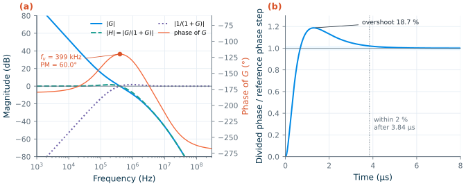
python3 pll_lab.py looppll_lab.pyreads the components of the third-order filter fromtools/figs/ch12_numbers.json(those of Worked example 12.1: \(R_1\) = 24.5 kΩ, \(C_1\) = 60.0 pF, \(C_2\) = 2.35 pF, \(R_3\) = 19.0 kΩ, \(C_3\) = 1.21 pF) and the calibrated \(K_{VCO}\) range, 103–167 MHz/V, from the same file; it designs for the range’s geometric centre, 131 MHz/V, not for the 96.9 MHz/V mean that step 1 measures at code 8. Its functionloop(), written with python-control [180], is the heart of the lab:import control as ct s = ct.tf("s") YA = C2*s + C1*s/(1 + R1*C1*s) # node A: C2 and the R1-C1 branch Z = 1/((YA + C3*s/(1 + R3*C3*s))*(1 + R3*C3*s)) # V_B / I_CP, Eq. (12.2) G = ICP*KVCO*Z/(N*s) # loop gain, Eq. (12.1) H = ct.feedback(G, 1) # reference phase -> divided phase E = ct.feedback(1, G) # VCO phase noise -> output gm, pm, wcg, wcp = ct.margin(G) # crossover wcp (rad/s) and phase margin ct.step_info(H) # overshoot, settling timeThe step prints \(f_u\) and the phase margin, the same for \(K_{VCO}\) 30 % low and high with the filter fixed, the zero and poles of \(Z(s)\) from
ct.zeros()andct.poles(), \(\vert Z\vert\) at \(f_{ref}\), the peaking of \(H\) and of \(1/(1+G)\), and the response of the divided phase to a step of the reference phase: its overshoot, and the time after which it stays within 2 % and within 0.1 %. For a linear loop the same response describes the VCO frequency after a step of the channel, so the 0.1 % time is a lock time. -
The noise budget.
python3 pll_lab.py noiseFirst it runs
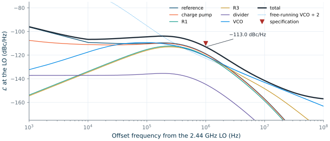
out/cp_noise.cir, Chapter 12’s charge pump with both sources on and its output held at 0.6 V (cp_netlist()of the chapter script), through an ngspicenoiseanalysis, and turns the output noise current into its duty-cycled effective value for a 0.5 ns reset pulse per 25 ns, Eq. (12.10). Then it shapes every source with the transfer functions of step 4, Eqs. (12.6)–(12.9): the TCXO (datasheet points of Section 12.3 [208]), the retimed divider (57.3 fs per edge, the chapter’s assumption) and the charge pump through \(NH\); the thermal noise of \(R_1\) and \(R_3\) through the filter’s noise transimpedances and \(2\pi K_{VCO}/s \cdot 1/(1+G)\); and the VCO through \(1/(1+G)\). The VCO’s free-running noise is Chapter 11’s simulated curve (pn.sim_curveinch11_numbers.json, every noise source, 1/f³ corner 254 kHz), scaled from 4.868 to 4.880 GHz. Everything is divided by four for the LO, the divide-by-two’s floor (−158.1 dBc/Hz, Chapter 13) is added, and the jitter is integrated from 10 kHz to 10 MHz with Eq. (12.11). -
Figures.
python3 pll_lab.py allruns both steps, stores the numbers underpllinlab_numbers.jsonand draws Figure L6.2 and Figure L6.3 intoout/.
Checkpoint
Table L6.1. Lab 6, Part A: the course VCO (SG13G2, tt, 27 °C; code 8, Vtune = 0.6 V unless stated). Tolerance: ±1 in the last digit shown, except where stated.
| Quantity | Lab 6 | Chapter 11 |
|---|---|---|
| Hand calculation: \(f_0\); \(Q_{tank}\), \(R_p\) (Eq. 11.4) | 4.88 GHz; 14.9, 907 Ω | |
| Hand calculation: \(V_A\) (Eq. 11.5); peak \(K_{VCO}\) (Eq. 11.7) | 0.692 V; 180 MHz/V | 0.692 V; 180 MHz/V |
| Frequency at the design point | 4.868 GHz | 4.868 GHz (Table 11.2) |
| Differential peak amplitude; per side; output common mode | 0.784 V; 0.392 V; 0.739 V | 0.784 V; 0.392 V; 0.739 V |
| Supply current, power | 0.639 mA, 0.766 mW | 0.639 mA, 0.766 mW |
| Coverage: code 15 at 0 V to code 0 at 1.2 V | 4.633–5.224 GHz | 4.633–5.224 GHz |
| Band of codes 0 / 8 / 15 over 0–1.2 V | 136 / 116 / 103 MHz | 136 / 116 / 103 MHz |
| Mean \(K_{VCO}\), codes 0 / 8 / 15 | 113 / 96.9 / 85.6 MHz/V | 113 / 96.9 / 85.6 MHz/V |
| Amplitude over the seven points | 0.745–0.861 V | 0.744–0.861 V (all tt points) |
| Tank: \(Q_{tank}\), \(R_p\), \(C\) (differential) | 14.9, 906 Ω, 537 fF | 14.9, 906 Ω, 537 fF |
| Q of spiral / bank / varactor / MIM / divider input | 17.8 / 21.6 / 98.3 / 394 / 12.2 | 17.8 / 21.6 / 98.3 / 394 / 12.2 |
| Share of the losses: spiral / bank (±0.5 points) | 83.8 / 10.4 % | 84 / 10 % |
Table L6.2. Lab 6, Part B: the course PLL (fref = 40 MHz, N = 122, ICP = 100 µA, KVCO = 131 MHz/V, third-order filter of Worked example 12.1). Phase noise in dBc/Hz at the 2.44 GHz LO; jitter from 10 kHz to 10 MHz. Tolerance: ±1 in the last digit shown, except where stated.
| Quantity | Lab 6 | Chapter 12 |
|---|---|---|
| Hand calculation: \(b\); zero; combined pole; \(R_1\) estimate | 3.73; 107 kHz; 1.49 MHz; 23.4 kΩ | 3.73; 107 kHz; 1.49 MHz; 23.4 kΩ |
| Hand calculation: TCXO floor in band, at the VCO / at the LO | −105.3 / −111.3 dBc/Hz | −105.3 / −111.3 dBc/Hz |
\(f_u\), phase margin (ct.margin) |
399 kHz, 60.0° | 400 kHz, 60.0° |
| \(K_{VCO}\) = 103 / 167 MHz/V (the calibrated range): \(f_u\), PM | 322 kHz, 59.4° / 496 kHz, 59.4° | 323 kHz, 59.4° / 496 kHz, 59.4° |
| Zero; poles of \(Z(s)\) (±0.1 MHz for the second pole) | 108 kHz; 1.75 MHz, 11.61 MHz | 108 kHz; 1.75 MHz, 11.6 MHz |
| \(\vert Z\vert\) at 40 MHz | 281 Ω | 282 Ω |
| Peaking of \(NH\) / of \(1/(1+G)\) | 1.72 / 1.77 dB | 1.72 dB |
| Step response: overshoot; peak time | 18.7 %; 1.30 µs | 18.7 % (Section 12.6) |
| Step response: within 2 % / within 0.1 % after | 3.84 / 6.48 µs | |
| Charge pump, both on: white noise, flicker corner | 6.74 pA/√Hz, 93.1 kHz | 6.74 pA/√Hz, 93.1 kHz |
| TCXO: 100 kHz / 1 MHz / 10 MHz; jitter | −110.1 / −118.8 / −157.0; 236 fs | −110.1 / −118.8 / −157.0; 236 fs (Table 12.2) |
| Charge pump | −110.5 / −119.2 / −157.4; 223 fs | −110.5 / −119.2 / −157.4; 223 fs |
| R1 | −115.2 / −120.6 / −158.8; 171 fs | −115.2 / −120.6 / −158.7; 171 fs |
| R3 | −116.0 / −120.9 / −148.3; 162 fs | −116.0 / −120.9 / −148.3; 162 fs |
| Divider | −136.0 / −144.6 / −182.8; 11.9 fs | −136.0 / −144.6 / −182.8; 11.9 fs |
| VCO (Chapter 11, simulated) | −109.4 / −120.9 / −143.1; 206 fs | −109.4 / −120.9 / −143.1; 206 fs |
| Total: 100 kHz / 1 MHz / 3 MHz / 10 MHz | −104.5 / −113.0 / −127.2 / −141.5 | −104.5 / −113.0 / −127.1 / −141.5 |
| Total: jitter, rms phase; margin at 1 MHz | 451 fs, 0.396°; 3.0 dB | 451 fs, 0.396°; 3.0 dB |
| VCO and TCXO alone: 1 MHz; jitter | −116.7 dBc/Hz; 313 fs |
Both parts reproduce their chapters. Part A’s seven transients give the same frequencies, amplitudes, currents and tuning gains as the 96 transients of Section 11.5 at those points; the shares of the tank losses differ by up to 0.4 points because this lab evaluates the admittances exactly at \(f_0\), while Chapter 11 interpolated them from a 50 MHz grid. In Part B, the filter components carry the three digits of Worked example 12.1, which moves the crossover to 399 kHz and a few contributions by up to 0.05 dB; nothing else changes beyond the last digit. Part B does not use the mean \(K_{VCO}\) that Part A measures at code 8 (96.9 MHz/V): it uses what the loop sees once the band calibration of Section 11.8 has chosen the code, 103–167 MHz/V, and designs for the centre, 131 MHz/V.
Questions
- The four passive elements of step 2 add up to 441 fF, but the spiral resonates with 537 fF at \(f_0\). Where are the other 96 fF, and why does the hand calculation’s 4.88 GHz still come out within 0.3 % of the simulation?
- The small-signal \(K_{VCO}\) peaks at 180 MHz/V, the transients give a mean of 96.9 MHz/V at code 8. Why are they so different (the pitfall of Section 11.5), and why does the loop designer use neither, but the 103–167 MHz/V of Section 11.8?
- The phase margin is 60° and yet the step response overshoots by 18.7 %, about twice what a second-order system with 60° of margin would give. What in the type-II loop’s closed-loop transfer function causes the extra overshoot?
- Free-running, the VCO divided by two would give −122.7 dBc/Hz at 1 MHz; inside the loop it contributes −120.9 dBc/Hz. Which transfer function makes the VCO worse at 1 MHz, and by how much should that be, from the peaking in Table L6.2?
- The total misses the specification only if the in-band sources rise by about 3 dB. Rank the reference, the charge pump and the resistors by what it would cost to improve each by 3 dB.
- A BLE channel hop leaves 150 µs between packets. With 6.5 µs to settle within 0.1 %, which other effect of a real synthesizer will dominate the lock time?
Extension
Part A. Run the slow corner of Section 11.5 for the bottom of the range: in out/vco_tune.cir, change mos_tt to mos_ss in both MOS .lib lines and cap_typ to cap_wcs, add .options temp=85, rerun ngspice with the printed command and analyse with python3 vco_lab.py tune --nosim. Compare code 15 at 0 V with Chapter 11’s 4.516 GHz and with the bottom of the course band.
Part B. Redesign the loop for \(I_{CP}\) = 200 µA, the next row of Table 12.1. Get the components from the chapter’s design routine (import ch12_pll_noise as C12; F = C12.design(icp=200e-6), then F.R1, F.C1, F.C2, F.R3, F.C3), put them and the new ICP into pll_lab.py, and double the charge pump’s noise current power in cp_noise(), since the cell is scaled at constant current density. Check loop first (still 400 kHz and 60°?), then noise: Table 12.1 gives −114.8 dBc/Hz at 1 MHz and 379 fs, for twice the capacitor area.