Chapter 3
Transmission Lines, the Smith Chart and S-Parameters
At radio frequencies a wire is no longer a node: a signal takes time to travel along it, and part of it reflects wherever the impedance changes. This chapter builds the language that RF engineers use for this, transmission lines, reflection coefficients, the Smith chart and S-parameters, and then uses it on an SG13G2 transistor: its gains, its stability, and how to measure it on a chip.
- Decide when an interconnect must be treated as a transmission line, and calculate its characteristic impedance, delay and attenuation.
- Calculate the reflection coefficient, VSWR and return loss of a load and the input impedance of a terminated line, and read a time-domain reflection.
- Use the Smith chart to move a load along a line and through series and shunt elements, and design a quarter-wave and an L-section match.
- Convert between Z, Y, ABCD and S-parameters, and compute the transducer, operating and available power gains, MSG, MAG and U of a transistor.
- Test a two-port for stability with K, μ and stability circles, and remove pad parasitics from on-chip measurements by open–short de-embedding.
Contents
3.1 When wires become transmission lines
In an analog circuit we assume that a wire has the same voltage everywhere along it. That holds while the signal’s period is long compared with the time the signal takes to travel along the wire. A signal travels at \(v_p = c/\sqrt{\varepsilon_{eff}}\), where \(\varepsilon_{eff}\) is the effective relative permittivity of the material around the conductors, so one period covers a wavelength
\[\lambda = \frac{v_p}{f} = \frac{c}{f\sqrt{\varepsilon_{eff}}}. \tag{3.1}\]When a wire is longer than about a tenth of a wavelength, its two ends differ in phase by more than 36°, and it must be treated as a transmission line [8, 7]. At 2.44 GHz, the centre of the course radio’s band, λ is 122.9 mm in free space and 60.7 mm in silicon dioxide (\(\varepsilon_r\) = 4.1). A tenth of that, 6 mm, is larger than most chips, so the wires inside a 2.4 GHz receiver can be modelled as lumped resistors, capacitors and inductors. The connections around the chip cannot: bond wires, package traces, the board trace to the antenna, cables and probes are lines, and every measurement is made through them. At 50 GHz (Chapter 17) λ in oxide is 2.96 mm, so a 0.3 mm interconnect on the chip is already λ/10, and the matching networks themselves are built from lines.
The telegrapher’s equations
A line is two conductors, a signal and its return. Cut it into short sections of length \(\Delta z\) (Figure 3.1). Each section has a series resistance \(R'\Delta z\) (the metal) and inductance \(L'\Delta z\) (the magnetic field around the current), and a shunt conductance \(G'\Delta z\) (losses in the dielectric and substrate) and capacitance \(C'\Delta z\) (the electric field between the conductors). The primes mark values per unit length. Kirchhoff’s laws across one section, in the limit \(\Delta z \to 0\), give the telegrapher’s equations for the phasors \(V(z)\) and \(I(z)\):
\[\frac{dV}{dz} = -(R' + j\omega L')\,I, \qquad \frac{dI}{dz} = -(G' + j\omega C')\,V. \tag{3.2}\]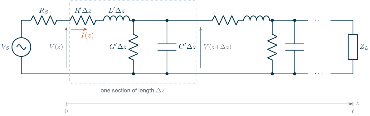
Eliminating \(I\) gives a wave equation, \(d^2V/dz^2 = \gamma^2 V\), whose solution is a wave travelling towards the load plus one travelling back, \(V(z) = V^+e^{-\gamma z} + V^-e^{+\gamma z}\).
Key equation · Propagation constant and characteristic impedance
\[\gamma = \alpha + j\beta = \sqrt{(R' + j\omega L')(G' + j\omega C')}, \qquad Z_c = \frac{V^+}{I^+} = \sqrt{\frac{R' + j\omega L'}{G' + j\omega C'}}. \tag{3.3}\]Each wave decays by \(e^{-\alpha z}\) and turns its phase by \(\beta z\), with \(\beta = 2\pi/\lambda\). A single wave has voltage \(Z_c\) times its current.
For a lossless line (\(R' = G' = 0\)) the characteristic impedance is real and frequency-independent, and the wave has no dispersion:
\[Z_0 = \sqrt{L'/C'}, \qquad v_p = 1/\sqrt{L'C'}. \tag{3.4}\]Worked example 3.1 · A 50 Ω line on the chip
Take a line with \(Z_0\) = 50 Ω and \(\varepsilon_{eff}\) = 4, so \(v_p = c/2\). From Eq. (3.4), \(L' = Z_0/v_p\) = 0.334 nH/mm and \(C' = 1/(Z_0v_p)\) = 0.133 pF/mm, and the delay is \(1/v_p\) = 6.67 ps/mm. A 5 mm line delays a signal by 33.3 ps. This chapter uses these values for its example lines; Chapter 7 extracts real ones for SG13G2’s top metals with electromagnetic simulation.
Loss and dispersion
On a chip, \(R'\) is not small: the top metals are a few micrometres thick, and the current crowds into their surface at gigahertz frequencies (the skin effect). When \(R' \ll \omega L'\) and \(G' \ll \omega C'\), Eq. (3.3) simplifies to
\[\alpha \approx \frac{R'}{2Z_0} + \frac{G'Z_0}{2}, \tag{3.5}\]independent of frequency. Below about \(R'/(2\pi L')\) the line is resistive-capacitive instead: \(\alpha\) falls with frequency, and \(Z_c\) becomes large and complex.
ngspice has two line elements [194]: T, a lossless line defined by \(Z_0\) and its delay, and LTRA, a lossy line defined by its \(R'\), \(L'\), \(G'\) and \(C'\) and solved by convolution with its impulse response [54]:
* lossless 50-ohm line, 0.5 ns delay
T1 in 0 out 0 Z0=50 TD=0.5n
* lossy line: per-metre R', L', G', C' and the length (here 10 ohm/mm, 5 mm)
O1 in 0 out 0 lline
.model lline LTRA R=10k L=333.3n G=0 C=133.3p LEN=5m
Figure 3.2a sends a 1 V step through 5 mm of the line of Worked example 3.1, with 50 Ω at both ends and \(R'\) = 0, 2 and 10 Ω/mm. The lossless line delivers a clean 0.5 V step after 33.3 ps. The lossy lines first jump to \(0.5\,e^{-\alpha\ell}\), with the high-frequency attenuation \(\alpha = R'/2Z_0\) of Eq. (3.5): 0.452 V and 0.303 V. They then creep up to the DC value of the resistive divider, \(50/(100 + R'\ell)\): 0.4545 V and 0.333 V. The slow tail is the resistive-capacitive part of the line at low frequencies. The exact solution of Eq. (3.3), computed in the frequency domain and transformed back, agrees with the ngspice transient to within 3 mV.
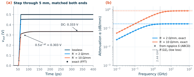
sp analysis through the ABCD parameters (Section 3.5), against Eq. (3.3) (lines) and the low-loss limit R′/2Z0 (dashed).Figure 3.2b shows the attenuation against frequency, extracted from an S-parameter simulation of each line. The two lines become “low loss” above \(R'/(2\pi L')\) = 0.955 GHz and 4.78 GHz. At 2.44 GHz the 2 Ω/mm line loses 0.171 dB/mm, close to its limit of 0.174 dB/mm, and has \(Z_c\) = 50.9 − j9.6 Ω. The 10 Ω/mm line loses 0.687 dB/mm (limit 0.869 dB/mm), and its characteristic impedance, 63.2 − j38.7 Ω, is far from the 50 Ω it was designed for; at 100 MHz it is 247 − j242 Ω. LTRA keeps \(R'\) and \(G'\) constant, so it leaves out the skin effect and the substrate loss that make real on-chip lines lossier at high frequencies; Chapter 7 adds them with electromagnetic simulation.
3.2 Reflection, standing waves and return loss
At the end of a line the ratio of voltage to current must equal the load impedance \(Z_L\). A single wave has the ratio \(Z_0\), so unless \(Z_L = Z_0\) a reflected wave must appear. Its ratio to the incident wave is the reflection coefficient
\[\Gamma_L = \frac{V^-}{V^+} = \frac{Z_L - Z_0}{Z_L + Z_0}. \tag{3.6}\]An open circuit reflects everything in phase (\(\Gamma_L\) = +1), a short circuit in antiphase (−1), and a matched load nothing (0). For any passive load \(\vert\Gamma_L\vert \le 1\).
The incident and reflected waves interfere, so on a mismatched line the voltage amplitude varies with position between \(\vert V^+\vert(1 + \vert\Gamma\vert)\) and \(\vert V^+\vert(1 - \vert\Gamma\vert)\), a standing wave. Three numbers describe the mismatch: the voltage standing-wave ratio, the return loss (how far the reflected power is below the incident power) and the mismatch loss (how much less power reaches the load than a matched load would get):
\[\mathrm{VSWR} = \frac{1 + \vert\Gamma\vert}{1 - \vert\Gamma\vert}, \qquad \mathrm{RL} = -20\log_{10}\vert\Gamma\vert, \qquad \mathrm{ML} = -10\log_{10}\left(1 - \vert\Gamma\vert^2\right). \tag{3.7}\]Table 3.1. Return loss, reflection coefficient, VSWR and mismatch loss (Eq. 3.7).
| Return loss (dB) | \(\vert\Gamma\vert\) | VSWR | Reflected power | Mismatch loss (dB) |
|---|---|---|---|---|
| 3 | 0.708 | 5.85 | 50.1 % | 3.0 |
| 6 | 0.501 | 3.01 | 25.1 % | 1.3 |
| 10 | 0.316 | 1.92 | 10.0 % | 0.46 |
| 15 | 0.178 | 1.43 | 3.16 % | 0.14 |
| 20 | 0.100 | 1.22 | 1.00 % | 0.044 |
| 30 | 0.0316 | 1.07 | 0.100 % | 0.0043 |
The course LNA must have \(\vert S_{11}\vert \le\) −10 dB, a return loss of at least 10 dB: 10 % of the power is reflected, and the mismatch loss is only 0.46 dB. The specification is less about the lost power than about what the reflection does to the blocks before the LNA: a band filter or an antenna is designed for a 50 Ω termination, and its response changes when the LNA reflects.
Reflections in the time domain
Reflections are easiest to see with a step. When a source with resistance \(R_S\) launches a step \(V_S\) into a line, the line looks like \(Z_0\) until a reflection comes back, so the wave \(V_1 = V_S Z_0/(Z_0 + R_S)\) starts down the line. At the load it reflects with \(\Gamma_L\), back at the source with \(\Gamma_S = (R_S - Z_0)/(R_S + Z_0)\), and so on. The bounce diagram of Figure 3.3a tracks the waves for \(R_S\) = 20 Ω, \(Z_0\) = 50 Ω, a delay \(T_D\) = 0.5 ns and \(R_L\) = 200 Ω: \(\Gamma_S\) = −0.429, \(\Gamma_L\) = 0.600 and \(V_1\) = 0.714 V. The load voltage, the sum of the waves that have arrived, steps to 1.143 V at \(T_D\), then 0.849, 0.925, 0.905 and 0.910 V, converging on the DC value of 0.909 V. The ngspice simulation (Figure 3.3b) gives the same plateaux to four digits; it differs from the exact solution by at most 5.4 mV, on the 10 ps edges.
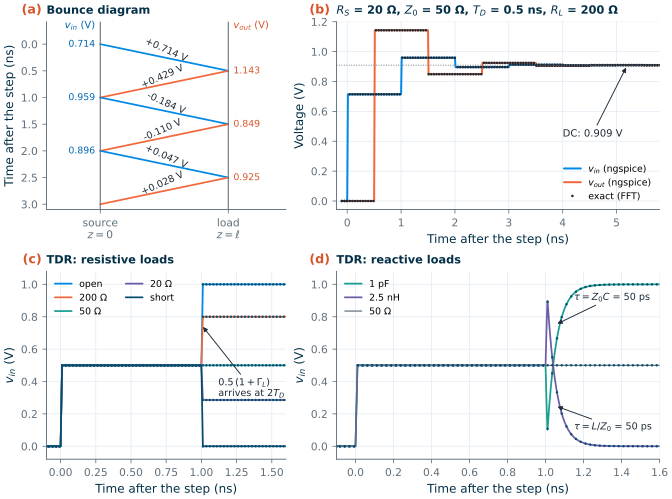
With a matched source the bouncing stops after one trip, and the input voltage reads the load directly. The step \(V_S/2\) goes out, and after the round trip \(2T_D\) the input voltage becomes
\[v_{in} = \frac{V_S}{2}\,(1 + \Gamma_L) \qquad (t > 2T_D,\ R_S = Z_0). \tag{3.8}\]This is time-domain reflectometry (TDR). In Figure 3.3c the open, 200 Ω, 50 Ω, 20 Ω and short loads give 1.000, 0.800, 0.500, 0.286 and 0 V, exactly Eq. (3.8). Reactive loads leave a shape (Figure 3.3d): a capacitor is a short at first and charges through \(Z_0\) with \(\tau = Z_0C\) (50 ps for 1 pF), and an inductor is an open at first and relaxes with \(\tau = L/Z_0\) (50 ps for 2.5 nH). A TDR trace of a packaged chip shows each bond wire as an inductive bump and each pad as a capacitive dip, at the time that locates it.
3.3 The terminated line and the quarter-wave transformer
Seen from a distance \(d\) before the load, the reflected wave has travelled \(2d\) further than the incident one. The reflection coefficient therefore turns by \(2\beta d\) (and shrinks by \(e^{-2\alpha d}\)), and so does the impedance:
Key equation · Input impedance of a terminated line
\[\Gamma(d) = \Gamma_L\,e^{-2\gamma d}, \qquad Z_{in}(d) = Z_0\,\frac{Z_L + jZ_0\tan\beta d}{Z_0 + jZ_L\tan\beta d} \quad \text{(lossless)}. \tag{3.9}\]
Derivation · Input impedance of a lossless line
With \(d\) measured from the load towards the source, \(V = V^+(e^{j\beta d} + \Gamma_L e^{-j\beta d})\) and \(I = (V^+/Z_0)(e^{j\beta d} - \Gamma_L e^{-j\beta d})\). Their ratio is \(Z_{in} = Z_0(1 + \Gamma_L e^{-2j\beta d})/(1 - \Gamma_L e^{-2j\beta d})\), which is the first form of Eq. (3.9). Substituting Eq. (3.6) for \(\Gamma_L\), multiplying out and dividing numerator and denominator by \(\cos\beta d\) gives the tangent form.
Three special cases matter. A line of \(\lambda/2\) repeats its load. A shorted or open line, a stub, is a pure reactance,
\[Z_{in}^{sc} = jZ_0\tan\beta d, \qquad Z_{in}^{oc} = -jZ_0\cot\beta d, \tag{3.10}\]inductive and capacitive respectively when shorter than \(\lambda/4\): the inductors and capacitors of millimetre-wave matching networks. And a line of \(\lambda/4\), with \(\tan\beta d \to \infty\), inverts its load, \(Z_{in} = Z_1^2/Z_L\). A quarter-wave line of impedance \(Z_1\) therefore matches a resistance \(R_L\) to \(Z_0\) when
\[Z_1 = \sqrt{Z_0R_L}, \tag{3.11}\]the quarter-wave transformer. It needs a resistive load; a complex load is first moved along a line to the point where its impedance is real.
Worked example 3.2 · Matching a capacitive load with lines
The load is 20 Ω in series with 1.63 pF, normalized \(z_L = Z_L/Z_0\) = 0.4 − j0.8 at 2.44 GHz, the kind of impedance a transistor input presents. Eq. (3.6) gives \(\Gamma_L\) = 0.620 at −97.1°: VSWR 4.27, return loss 4.15 dB, mismatch loss 2.11 dB.
- A 50 Ω line of \(d\) = 0.115λ turns \(\Gamma\) by \(2\beta d\) = 82.9° to −180°, where the impedance is real and smallest: \(Z_0/\mathrm{VSWR}\) = 11.7 Ω. (At the opposite point it is \(Z_0\cdot\mathrm{VSWR}\) = 213 Ω.)
- A quarter-wave line of \(Z_1 = \sqrt{50 \times 11.7}\) = 24.2 Ω (Eq. 3.11) turns 11.7 Ω into 50 Ω.
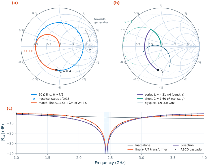
ngspice confirms the match (Figure 3.4c): \(\vert S_{11}\vert\) at 2.44 GHz is −118 dB, numerically zero, and stays below −10 dB from 2.23 to 2.68 GHz, 18.5 % of the centre frequency. On a chip, with \(\varepsilon_{eff}\) = 4, the two lines are 7.07 mm and 15.4 mm long, larger than the chip. At 2.4 GHz on-chip matching uses lumped elements instead (Section 3.4); at 50 GHz a quarter wave is only 0.75 mm, and lines become practical.
3.4 The Smith chart
Impedances fill an infinite half-plane, which is awkward to draw. Reflection coefficients of passive loads fill a unit circle. P. H. Smith’s idea [44] was to plot \(\Gamma\) and draw on it the lines of constant resistance and reactance. With the normalized impedance \(z = Z/Z_0 = r + jx\),
\[\Gamma = \frac{z - 1}{z + 1}, \qquad z = \frac{1 + \Gamma}{1 - \Gamma}. \tag{3.12}\]This mapping turns the lines of constant \(r\) and of constant \(x\) into circles:
\[\begin{gathered} \text{constant } r:\ \text{centre } \left(\tfrac{r}{1 + r}, 0\right),\ \text{radius } \tfrac{1}{1 + r}; \\ \text{constant } x:\ \text{centre } \left(1, \tfrac{1}{x}\right),\ \text{radius } \tfrac{1}{\vert x\vert}. \end{gathered} \tag{3.13}\]The centre of the chart is the matched load, the left end of the horizontal axis the short and the right end the open; inductive impedances lie in the upper half, capacitive ones in the lower half. The admittance \(y = 1/z\) has reflection coefficient \(-\Gamma\), so the admittance chart, with circles of constant conductance \(g\) and susceptance \(b\), is the same chart turned by 180° (Figure 3.4b, dotted). Every matching network can be drawn as a path on the two charts together.
Moving along a line. By Eq. (3.9), a lossless line turns \(\Gamma\) clockwise (“towards the generator”) about the centre by \(2\beta d\), at constant \(\vert\Gamma\vert\); half a wavelength is one full turn. A lossy line spirals inwards. Figure 3.4a draws the circle of the load of Worked example 3.2 and the ngspice input reflection coefficients of 50 Ω lines of 0 to \(\lambda/2\) in steps of \(\lambda/16\): each step turns \(\Gamma\) by 45°, from −97.1° to −142.1°, 172.9° and on, back to −97.1° at \(\lambda/2\), all at \(\vert\Gamma\vert\) = 0.620. The orange path is the quarter-wave match: along the circle to 11.7 Ω, then along the circle of the 24.2 Ω transformer to the centre.
Adding series and shunt elements. A series reactance changes \(x\) and leaves \(r\) alone, so it moves the point along a circle of constant resistance; a shunt susceptance moves it along a circle of constant conductance (Table 3.2).
Table 3.2. How lumped elements move an impedance on the Smith chart.
| Element | Moves along a circle of constant | Direction | Towards |
|---|---|---|---|
| Series inductor | resistance \(r\) | clockwise | upper half (inductive) |
| Series capacitor | resistance \(r\) | counter-clockwise | lower half (capacitive) |
| Shunt capacitor | conductance \(g\) | clockwise | lower half (capacitive) |
| Shunt inductor | conductance \(g\) | counter-clockwise | upper half (inductive) |
Worked example 3.3 · An L-section for the same load
Start at \(z_L\) = 0.4 − j0.8 (Figure 3.4b). A series inductor moves the point clockwise along the circle \(r\) = 0.4 until it reaches the circle \(g\) = 1, at \(z\) = 0.4 + j0.490: \(x\) changes by 1.290, so \(\omega L\) = 64.5 Ω and \(L\) = 4.21 nH. There \(y\) = 1 − j1.225, so a shunt capacitor with \(b\) = 1.225 cancels the susceptance and lands on the centre: \(C = b/(\omega Z_0)\) = 1.60 pF. ngspice gives \(\vert S_{11}\vert\) = −108 dB at 2.44 GHz.
Line + λ/4 transformer L-section Elements 0.115λ of 50 Ω, λ/4 of 24.2 Ω 4.21 nH series, 1.60 pF shunt Size on chip at 2.44 GHz 7.07 mm + 15.4 mm of line two components \(\vert S_{11}\vert\) < −10 dB 2.23–2.68 GHz (18.5 %) 2.14–2.72 GHz (23.8 %) \(\vert S_{11}\vert\) < −15 dB 9.97 % 12.9 % \(\vert S_{11}\vert\) < −20 dB 5.54 % 7.19 % Both cover the 2.400–2.4835 GHz band with a wide margin. Their bandwidth is set mostly by the load itself, whose reactance is twice its resistance; the line version is narrower because its 0.365λ of line adds frequency dependence of its own. Chapter 8 designs matching networks systematically, including their bandwidth limits and losses.
The ngspice results and a calculation that cascades the ABCD matrices of Section 3.5 agree to within \(10^{-5}\) in \(\Gamma\), the print precision of the simulator (Figure 3.4c).
Try the chart. Drag the orange load anywhere on the chart and read its reflection, VSWR and mismatch loss. Then add two elements: a series element moves the point along a circle of constant resistance, a shunt element along a circle of constant conductance, and two of them can reach the centre from almost anywhere. “Find an L-match” solves that two-element network exactly, the subject of Chapter 8.
3.5 Two-port networks: Z, Y, ABCD and S
An amplifier, a filter or a transistor is a two-port: a network with an input and an output port, each a pair of terminals with a voltage across it and a current through it (Figure 3.5). Four parameters relate the four quantities, in several equivalent ways. The impedance and admittance matrices give the voltages from the currents and the reverse,
\[\begin{bmatrix} V_1 \\ V_2 \end{bmatrix} = \begin{bmatrix} Z_{11} & Z_{12} \\ Z_{21} & Z_{22} \end{bmatrix}\begin{bmatrix} I_1 \\ I_2 \end{bmatrix}, \qquad \begin{bmatrix} I_1 \\ I_2 \end{bmatrix} = \mathbf{Y}\begin{bmatrix} V_1 \\ V_2 \end{bmatrix}, \quad \mathbf{Y} = \mathbf{Z}^{-1}, \tag{3.14}\]measured with the other port open (\(Z\)) or shorted (\(Y\)). The ABCD (chain) matrix relates the input to the output, with \(I_2\) taken flowing out of port 2,
\[\begin{bmatrix} V_1 \\ I_1 \end{bmatrix} = \begin{bmatrix} A & B \\ C & D \end{bmatrix}\begin{bmatrix} V_2 \\ I_2 \end{bmatrix}, \qquad \mathbf{M}_{cascade} = \mathbf{M}_1\mathbf{M}_2\cdots, \tag{3.15}\]so the matrix of a cascade is the product of the matrices of its stages. A line of length \(\ell\) has \(A = D = \cosh\gamma\ell\), \(B = Z_c\sinh\gamma\ell\) and \(C = \sinh(\gamma\ell)/Z_c\); a series impedance \(Z\) has \(B = Z\) and a shunt admittance \(Y\) has \(C = Y\) (the other entries 1 on the diagonal and 0 elsewhere). This is how Figure 3.2b extracted \(\gamma\) from a simulation: \(\cosh\gamma\ell = A\) and \(Z_c = \sqrt{B/C}\).
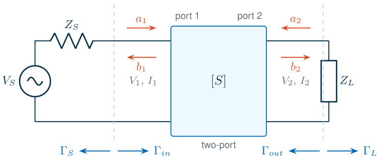
At radio frequencies \(Z\) and \(Y\) are hard to measure. A good open or short is difficult to make over a wide band, a transistor with an open or shorted port may oscillate, and voltages and currents cannot be measured directly at a port, only through the cables. Waves can: a directional coupler separates the wave going into a port from the wave coming out. The scattering parameters therefore describe a network with every port terminated in a reference impedance \(Z_0\), usually 50 Ω, using the power waves of Kurokawa [45]:
\[a = \frac{V + Z_0I}{2\sqrt{Z_0}}, \qquad b = \frac{V - Z_0I}{2\sqrt{Z_0}}, \qquad \begin{bmatrix} b_1 \\ b_2 \end{bmatrix} = \begin{bmatrix} S_{11} & S_{12} \\ S_{21} & S_{22} \end{bmatrix}\begin{bmatrix} a_1 \\ a_2 \end{bmatrix}. \tag{3.16}\]\(\vert a\vert^2/2\) and \(\vert b\vert^2/2\) are the powers of the waves. \(S_{11}\) is the input reflection coefficient with port 2 matched (\(a_2\) = 0), \(S_{21}\) the forward transmission, so \(\vert S_{21}\vert^2\) is the power gain between 50 Ω terminations; \(S_{12}\) is the reverse transmission (the isolation of an amplifier) and \(S_{22}\) the output reflection coefficient. The parameter sets convert into one another [46, 8]:
\[\begin{gathered} \mathbf{Z} = Z_0(\mathbf{I} + \mathbf{S})(\mathbf{I} - \mathbf{S})^{-1}, \qquad \mathbf{Y} = \frac{1}{Z_0}(\mathbf{I} - \mathbf{S})(\mathbf{I} + \mathbf{S})^{-1}, \\ \mathbf{S} = (\mathbf{Z} - Z_0\mathbf{I})(\mathbf{Z} + Z_0\mathbf{I})^{-1}, \end{gathered} \tag{3.17}\]with \(\mathbf{I}\) the unit matrix.
Conversion · ABCD from S (equal real reference impedances Z0)
\[A = \frac{(1 + S_{11})(1 - S_{22}) + S_{12}S_{21}}{2S_{21}}, \qquad B = Z_0\,\frac{(1 + S_{11})(1 + S_{22}) - S_{12}S_{21}}{2S_{21}},\] \[C = \frac{1}{Z_0}\,\frac{(1 - S_{11})(1 - S_{22}) - S_{12}S_{21}}{2S_{21}}, \qquad D = \frac{(1 - S_{11})(1 + S_{22}) + S_{12}S_{21}}{2S_{21}}.\]They follow from Eq. (3.16) by writing \(V\) and \(I\) at each port in terms of \(a\) and \(b\) and eliminating the waves; Frickey [46] gives the general case with complex reference impedances.
Terminate port 2 in a load \(\Gamma_L\) instead of \(Z_0\), and part of the output wave returns into the network and, through \(S_{12}\), to the input:
Key equation · Input and output reflection coefficients of a terminated two-port
\[\Gamma_{in} = S_{11} + \frac{S_{12}S_{21}\Gamma_L}{1 - S_{22}\Gamma_L}, \qquad \Gamma_{out} = S_{22} + \frac{S_{12}S_{21}\Gamma_S}{1 - S_{11}\Gamma_S}. \tag{3.18}\]The input of a two-port depends on its load, and its output on its source, unless \(S_{12}\) = 0 (a unilateral two-port).
S-parameters of an SG13G2 transistor
ngspice’s sp analysis (Chapter 2) computes the S-, Y- and Z-parameters of a circuit whose ports are voltage sources with a portnum and a reference impedance z0. The transistor of this chapter is an sg13_lv_nmos with 20 fingers of 2 µm (W = 40 µm) at L = 0.13 µm, biased at \(I_D\) = 2.00 mA (\(V_{GS}\) = 0.700 V) and \(V_{DS}\) = 0.6 V through ideal bias tees. rfmode=1 switches on the RF part of the IHP model: gate resistance, substrate resistances and non-quasi-static effects [191].
* ports 1 and 2 with bias tees (1 F, 1 H) around the common-source nMOS
V1 p1 0 dc 0 ac 1 portnum 1 z0 50
C1 p1 g 1
LG g gb 1
VG gb 0 0.700
V2 p2 0 dc 0 ac 1 portnum 2 z0 50
C2 p2 d 1
LD d db 1
VD db 0 0.6
XM1 d g 0 0 sg13_lv_nmos W=40u L=0.13u ng=20 rfmode=1
.control
sp dec 40 97.14e6 100e9
.endc
Common pitfall · Too many ports in one
sprunngspice’s
spanalysis needs at least two ports, and its run time grows very steeply with the number of ports. Simulate independent test structures in separate runs instead of one netlist with many ports; the script of this chapter uses at most four ports per run.
Worked example 3.4 · From S to Y: what the transistor looks like at 2.44 GHz
The simulation gives \(S_{11}\) = 0.994 ∠ −6.4°, \(S_{21}\) = 1.402 ∠ 171.1° (2.94 dB), \(S_{12}\) = 0.0300 ∠ 82.7° (−30.5 dB) and \(S_{22}\) = 0.910 ∠ −6.0°. Eq. (3.17) converts them to Y-parameters, which map onto the small-signal model of The Art of Analog IC Design:
- \(Y_{11}\) = 0.035 + j0.892 mS: an input capacitance Im\((Y_{11})/\omega\) = 58.2 fF in series with 44.3 Ω, mostly the gate resistance of this layout.
- \(Y_{21}\) = 14.72 − j0.90 mS: its real part is the transconductance; the operating point gives \(g_m\) = 14.74 mS.
- \(Y_{12}\) = −0.010 − j0.316 mS: the gate–drain capacitance, \(C_{gd} = -\mathrm{Im}(Y_{12})/\omega\) = 20.6 fF.
- \(Y_{22}\) = 0.92 + j0.82 mS: an output conductance of 0.92 mS (the operating point’s \(g_{ds}\) is 0.83 mS) in parallel with the drain capacitances.
\(S_{11}\) is almost 1: in a 50 Ω system the gate at 2.44 GHz is nearly an open circuit; with a 50 Ω load the input impedance is 52.2 − j896 Ω. This is why an LNA needs an input matching network (Chapter 9).
3.6 Power gains
“Gain” is ambiguous for a two-port between arbitrary terminations, so RF design uses three power gains [9, 8]. The transducer gain compares the power delivered to the load with the power available from the source, the gain the amplifier actually provides:
Key equation · Transducer power gain
\[G_T = \frac{P_L}{P_{avs}} = \frac{(1 - \vert\Gamma_S\vert^2)\,\vert S_{21}\vert^2\,(1 - \vert\Gamma_L\vert^2)}{\vert 1 - \Gamma_S\Gamma_{in}\vert^2\,\vert 1 - S_{22}\Gamma_L\vert^2}. \tag{3.19}\]Between 50 Ω terminations (\(\Gamma_S = \Gamma_L\) = 0) it is \(\vert S_{21}\vert^2\).
The operating power gain \(G_P = P_L/P_{in}\) divides by the power that actually enters the input, so it does not depend on the source; the available gain \(G_A = P_{avn}/P_{avs}\) assumes a conjugately matched load, so it does not depend on the load:
\[G_P = \frac{\vert S_{21}\vert^2(1 - \vert\Gamma_L\vert^2)}{(1 - \vert\Gamma_{in}\vert^2)\,\vert 1 - S_{22}\Gamma_L\vert^2}, \qquad G_A = \frac{\vert S_{21}\vert^2(1 - \vert\Gamma_S\vert^2)}{\vert 1 - S_{11}\Gamma_S\vert^2\,(1 - \vert\Gamma_{out}\vert^2)}. \tag{3.20}\]For the transistor at 2.44 GHz between 50 Ω terminations, \(G_T\) = 2.94 dB, \(G_P\) = 21.9 dB and \(G_A\) = 10.6 dB. They differ so much because the input is almost purely reactive: very little of the available power enters the gate, and what does is amplified a lot (\(G_P\)); and the 50 Ω load is far from the output’s conjugate (\(G_A > G_T\)). \(G_T\) is the only one of the three that a 50 Ω test bench measures directly.
The unilateral approximation. If \(S_{12}\) were zero, the input and output could be matched separately, and the best transducer gain would be
\[G_{TU,max} = \frac{\vert S_{21}\vert^2}{(1 - \vert S_{11}\vert^2)(1 - \vert S_{22}\vert^2)}, \qquad u = \frac{\vert S_{11}S_{12}S_{21}S_{22}\vert}{(1 - \vert S_{11}\vert^2)(1 - \vert S_{22}\vert^2)}, \tag{3.21}\]where the unilateral figure of merit \(u\) bounds the error: the true maximum lies between \(G_{TU,max}/(1 + u)^2\) and \(G_{TU,max}/(1 - u)^2\) when \(u < 1\). For our transistor \(G_{TU,max}\) = 29.5 dB, but \(u\) = 17.2, so the approximation is meaningless. For example, matching the output conjugately, \(\Gamma_L = S_{22}^*\) = 0.910 ∠ 6.0°, gives by Eq. (3.18) \(\Gamma_{in}\) = 1.003 ∠ −19.1°. A magnitude above 1 means the input reflects more power than it receives, a negative input resistance: with a suitable source the stage would oscillate. Section 3.7 shows why.
Maximum available and maximum stable gain. When a two-port is unconditionally stable (Section 3.7), its input and output can be conjugately matched at the same time, and the transducer gain is then the maximum available gain (MAG). When it is not, no such match exists, and the useful number is the maximum stable gain (MSG): the MAG of the device after just enough resistive loss has been added to make it marginally stable [49]:
\[\mathrm{MSG} = \left\vert\frac{S_{21}}{S_{12}}\right\vert, \qquad \mathrm{MAG} = \left\vert\frac{S_{21}}{S_{12}}\right\vert\left(K - \sqrt{K^2 - 1}\right) \quad (K > 1), \tag{3.22}\]with the stability factor \(K\) of Eq. (3.24). A third figure of merit is Mason’s unilateral power gain [47, 48], the gain of the device made unilateral with lossless feedback and then matched:
\[U = \frac{\vert Y_{21} - Y_{12}\vert^2}{4\left(\mathrm{Re}\,Y_{11}\,\mathrm{Re}\,Y_{22} - \mathrm{Re}\,Y_{12}\,\mathrm{Re}\,Y_{21}\right)}. \tag{3.23}\]\(U\) does not change when lossless reciprocal networks are added around the device, so it measures the device alone; the frequency where \(U\) = 1 is the maximum oscillation frequency \(f_{max}\), and the frequency where the short-circuit current gain \(\vert h_{21}\vert = \vert Y_{21}/Y_{11}\vert\) reaches 1 is the transit frequency \(f_T\) (Chapter 6).
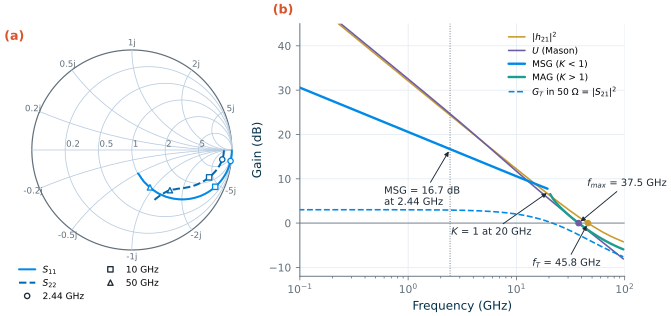
sg13_lv_nmos, W = 40 µm (20 × 2 µm), L = 0.13 µm, rfmode=1, ID = 2 mA, VDS = 0.6 V, ngspice sp from 0.1 to 97 GHz. (a) S11 and S22. (b) |h21|², Mason's U, the maximum stable gain (where K < 1) and maximum available gain (K > 1), and |S21|², the transducer gain between 50 Ω terminations.Figure 3.6 puts these together for our transistor. At 2.44 GHz the MSG is 16.7 dB and \(U\) is 24.7 dB. MSG falls at 10 dB per decade (as \(\vert S_{21}/S_{12}\vert \propto 1/f\)) until \(K\) reaches 1 at 20.0 GHz; above that the device is unconditionally stable and the curve continues as MAG. \(\vert h_{21}\vert^2\) and \(U\) fall at 20 dB per decade and give \(f_T\) = 45.8 GHz and \(f_{max}\) = 37.5 GHz. Here \(f_{max}\) is below \(f_T\) because of the 44.3 Ω series input resistance of this layout, mostly gate resistance; Chapter 6 shows how the layout of an RF transistor raises it.
What this means for your design
Quote \(G_T\) in the terminations the block really has; use MSG or MAG and \(U\) to judge what a device can deliver. An MSG of 16.7 dB at 2.44 GHz leaves little room for the course LNA’s 15 dB of gain once the matching networks and their losses are added. Chapter 9 uses a cascode, which reduces \(S_{12}\).
3.7 Stability
An amplifier oscillates when one of its ports reflects more power than it receives, \(\vert\Gamma_{in}\vert > 1\) or \(\vert\Gamma_{out}\vert > 1\): the port then has a negative resistance, which can cancel the loss of a resonant termination. A two-port is unconditionally stable at a frequency if no passive source and load (\(\vert\Gamma_S\vert, \vert\Gamma_L\vert < 1\)) make either magnitude reach 1, and potentially unstable otherwise. Two equivalent tests use only the S-parameters:
Key equation · Unconditional stability
\[\begin{gathered} K = \frac{1 - \vert S_{11}\vert^2 - \vert S_{22}\vert^2 + \vert\Delta\vert^2}{2\,\vert S_{12}S_{21}\vert} > 1 \ \text{ and } \ \vert\Delta\vert < 1, \\ \Delta = S_{11}S_{22} - S_{12}S_{21}; \qquad \text{or} \quad \mu = \frac{1 - \vert S_{11}\vert^2}{\vert S_{22} - \Delta S_{11}^*\vert + \vert S_{12}S_{21}\vert} > 1. \end{gathered} \tag{3.24}\]
The first is Rollett’s [49]; the second, by Edwards and Sinsky [50], needs a single number and has a geometric meaning: \(\mu\) is the distance from the centre of the Smith chart to the nearest load that makes \(\vert\Gamma_{in}\vert\) = 1, so a larger \(\mu\) means more margin. (A companion factor \(\mu'\), with the ports swapped, does the same for the source.)
Stability circles. By Eq. (3.18), the loads for which \(\vert\Gamma_{in}\vert\) = 1 lie on a circle in the \(\Gamma_L\) plane, and the sources for which \(\vert\Gamma_{out}\vert\) = 1 on a circle in the \(\Gamma_S\) plane [9]:
\[\begin{gathered} C_L = \frac{(S_{22} - \Delta S_{11}^*)^*}{\vert S_{22}\vert^2 - \vert\Delta\vert^2}, \qquad r_L = \frac{\vert S_{12}S_{21}\vert}{\left\vert\,\vert S_{22}\vert^2 - \vert\Delta\vert^2\right\vert}; \\ C_S = \frac{(S_{11} - \Delta S_{22}^*)^*}{\vert S_{11}\vert^2 - \vert\Delta\vert^2}, \qquad r_S = \frac{\vert S_{12}S_{21}\vert}{\left\vert\,\vert S_{11}\vert^2 - \vert\Delta\vert^2\right\vert}. \end{gathered} \tag{3.25}\]Which side is unstable? If \(\vert S_{11}\vert < 1\), a matched load (\(\Gamma_L\) = 0) is stable, so the side of the load circle that contains the centre of the chart is the stable one; likewise for the source circle when \(\vert S_{22}\vert < 1\).
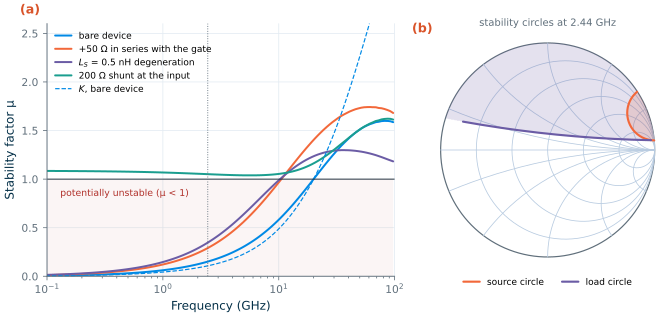
At 2.44 GHz our transistor has \(K\) = 0.108, \(\vert\Delta\vert\) = 0.907 and \(\mu\) = 0.151: potentially unstable. Figure 3.7b shows why. The load circle has its centre at 11.37 ∠ 84.0° and a radius of 11.22, so inside the chart it looks almost like a straight line, passing 0.151 from the centre (the value of \(\mu\)). Its inside, which does not contain the centre, is unstable: most inductive loads make \(\vert\Gamma_{in}\vert > 1\). This is the Miller effect at work: through \(C_{gd}\), an inductive load turns into a negative resistance at the gate. The source circle (centre 1.059 ∠ 19.1°, radius 0.257) cuts off a small region near the open circuit: a high, slightly inductive source impedance makes \(\vert\Gamma_{out}\vert > 1\). The conjugate load of Section 3.6, \(S_{22}^*\), lies just inside the load circle, which is why it gave \(\vert\Gamma_{in}\vert\) = 1.003.
Stabilizing the transistor. Figure 3.7a and Table 3.3 compare three common fixes. A 50 Ω resistor in series with the gate, or 0.5 nH of source degeneration, lowers the upper edge of the potentially unstable band: \(\mu\) crosses 1 at 10.5 GHz and 10.3 GHz instead of 20.0 GHz. The series resistor leaves the MSG unchanged, because a series element at a port changes neither \(Z_{21}\) nor \(Z_{12}\) and \(\vert S_{21}/S_{12}\vert = \vert Z_{21}/Z_{12}\vert\), but its loss lowers \(U\) from 24.7 to 21.0 dB. Neither helps at low frequencies: there the gate is an open circuit, \(1 - \vert S_{11}\vert^2 \to 0\), and \(\mu \to 0\) whatever is put in series with it. Only a resistance across the input makes \(\vert S_{11}\vert\) less than 1 at low frequencies. With 200 Ω from the gate to ground (AC-coupled, so the bias is unchanged), \(\mu\) stays above 1 at every frequency (its minimum is 1.039 at 5.8 GHz), and the transistor is unconditionally stable, at the price of 5.91 dB of maximum gain (a MAG of 10.8 dB instead of an MSG of 16.7 dB) and of the noise of the resistor (Chapter 4).
Table 3.3. The SG13G2 nMOS of Figure 3.6 at 2.44 GHz, alone and with three stabilizing elements (ngspice sp, tt, 27 °C).
| Bare device | +50 Ω in series with the gate | \(L_S\) = 0.5 nH | 200 Ω shunt at the input | |
|---|---|---|---|---|
| \(\vert S_{11}\vert\) (dB) | −0.056 | −0.109 | −0.131 | −4.48 |
| \(G_T\) in 50 Ω, \(\vert S_{21}\vert^2\) (dB) | 2.94 | 2.87 | 2.83 | 1.01 |
| \(K\) / \(\mu\) | 0.108 / 0.151 | 0.212 / 0.291 | 0.252 / 0.347 | 2.08 / 1.051 |
| MSG or MAG (dB) | 16.7 (MSG) | 16.7 (MSG) | 16.7 (MSG) | 10.8 (MAG) |
| \(U\) (dB) | 24.7 | 21.0 | 24.6 | 10.6 |
| Unconditionally stable (\(\mu\) > 1) | above 20.0 GHz | above 10.5 GHz | above 10.3 GHz | at all frequencies |
An LNA does not have to be unconditionally stable on its own; it must be stable with the source and load it will actually see, which Chapter 9 checks with its input match and cascode in place. But the antenna, the package and the probes of a test set-up all present impedances that can wander far from 50 Ω, and an amplifier that is unconditionally stable at every frequency cannot oscillate with any of them. Check \(\mu\) over the whole frequency range of the device, not only in the band: the bare transistor here is most nearly unstable at the lowest frequencies.
3.8 Measuring S-parameters on chip
A vector network analyser (VNA) measures S-parameters: it sends a wave into each port in turn and measures, through directional couplers, the amplitude and phase of the waves coming back from every port. The cables, connectors and probes between the instrument and the chip have their own reflections and losses, which a calibration removes: measuring known standards (short, open, load and thru, or transmission lines) on a calibration substrate moves the reference plane of the measurement to the tips of the probes [8, 10].
On the chip, the probes land on ground–signal–ground (GSG) pads (Figure 3.8a). Between the probe tips and the device there is still a pad on each port, with capacitance to the substrate and coupling to the other pad, and a feed line with series resistance and inductance. For a small RF transistor these parasitics are as large as the device’s own capacitances. They are removed by de-embedding: the same pads and feeds are laid out twice more on the chip as dummies, an open (the device left out) and a short (the feeds shorted to ground where the device would be). The open–short method [51] assumes that the pads are a shunt admittance at the outer plane, removed in Y-parameters, and the feeds a series impedance inside it, removed in Z-parameters:
\[\mathbf{Y}_{DUT} = \left[(\mathbf{Y}_{meas} - \mathbf{Y}_{open})^{-1} - (\mathbf{Y}_{short} - \mathbf{Y}_{open})^{-1}\right]^{-1}. \tag{3.26}\]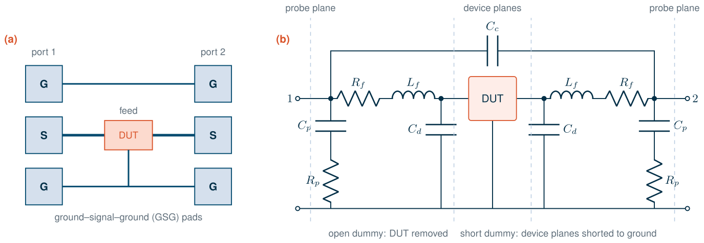
To see how well this works, the script simulates four structures with the transistor of Figure 3.6: the transistor alone (the reference), the transistor inside the pad model of Figure 3.8b (what the probes would measure), the open dummy and the short dummy. The capacitance \(C_d\) at the device end of the feeds deliberately breaks the method’s assumption: open–short treats it as part of the shunt pads, although it sits behind \(L_f\). Figure 3.9 and Table 3.4 compare the raw, open-only and open–short de-embedded results with the reference.
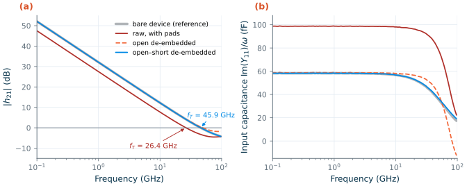
Table 3.4. The transistor seen through the pads of Figure 3.8, with and without de-embedding (ngspice sp; errors relative to the bare device).
| Bare device | Raw, with pads | Open de-embedded | Open–short de-embedded | |
|---|---|---|---|---|
| Input capacitance at 2.44 GHz | 58.2 fF | 98.6 fF | 58.6 fF | 58.1 fF |
| Series input resistance Re(1/\(Y_{11}\)) at 2.44 GHz | 44.3 Ω | 17.3 Ω | 41.7 Ω | 44.5 Ω |
| Error of \(Y_{11}\) at 2.44 GHz | – | 69.5 % | 0.84 % | 0.055 % |
| Error of \(Y_{11}\) / \(Y_{21}\) at 50 GHz | – | 109 % / 60.5 % | 40.3 % / 56.3 % | 2.99 % / 3.08 % |
| \(f_T\) | 45.8 GHz | 26.4 GHz | 49.4 GHz | 45.9 GHz |
| \(f_{max}\) | 37.5 GHz | 32.7 GHz | 36.3 GHz | 37.4 GHz |
The raw measurement adds 40.5 fF of pad, coupling and feed capacitance to the input, and underestimates \(f_T\) by 42.3 %: 26.4 GHz instead of 45.8 GHz. Subtracting the open removes almost all of the error at 2.44 GHz (0.84 % in \(Y_{11}\)), but the feeds remain in series, so \(f_T\) comes out 7.86 % too high and the input resistance too low. Open–short de-embedding recovers \(f_T\) to within 0.153 % and the input capacitance to within 0.052 %. Its residual error, 3 % at 50 GHz and 11.6 % in \(Y_{11}\) at 97 GHz, comes from \(C_d\), which the method puts on the wrong side of \(L_f\). Better dummies and methods, such as three-step de-embedding [52, 53], calibration on the chip itself, and electromagnetic models of the pads, handle such distributed parasitics at millimetre-wave frequencies (Chapter 18). Note also that the pads change the DC bias: the drain current drops from 2.000 to 1.998 mA because the feed resistance carries it.
Try it · The S-parameter script
Every number in this chapter comes from
tools/figs/ch03_sparams.py:python3 tools/figs/ch03_sparams.py tran lossy smith device deembed(helpers intools/figs/_ch03_rf.py). Three experiments: (1) insmith_part, change the loadZL0to 0.2 − j1.0, a higher-Q load: how much narrower do both matches become? (2) InVARIANTS, raise the shunt input resistor from 200 Ω to 500 Ω: is the transistor still unconditionally stable, and how much MAG do you win back? (3) InPAD, setcdto zero: does open–short de-embedding become exact?
- A wire longer than about λ/10 is a transmission line: Z0 = √(L′/C′) and vp = 1/√(L′C′) when lossless. At 2.44 GHz that means the connections around the chip; at 50 GHz the wires on it too.
- A load reflects ΓL = (ZL − Z0)/(ZL + Z0); a 10 dB return loss reflects 10 % of the power. A step shows each reflection at its round-trip time, and its shape shows what caused it.
- On the Smith chart a lossless line turns Γ clockwise by 2βd, a series element moves along a circle of constant r and a shunt element along a circle of constant g. A λ/4 transformer and an L-section both match 20 Ω + 1.63 pF at 2.44 GHz, with 18.5 % and 23.8 % bandwidth for a 10 dB return loss.
- S-parameters describe a network with 50 Ω on every port; Γin depends on the load unless S12 = 0. The SG13G2 nMOS (40 µm, 2 mA) has an MSG of 16.7 dB at 2.44 GHz, fT = 45.8 GHz and fmax = 37.5 GHz.
- The transistor is potentially unstable up to 20 GHz (μ = 0.151 at 2.44 GHz); series gate resistance and degeneration help only at high frequencies, while a resistor across the input makes it unconditionally stable at the cost of gain.
- On chip, the pads hide the device: they lower the apparent fT by 42 %, and open–short de-embedding recovers it to within 0.2 %.
Further reading
- D. M. Pozar, Microwave Engineering [8]: transmission lines, the Smith chart, network parameters and their conversions, and amplifier gain and stability, with many worked problems; G. Gonzalez [9] for power gains, stability circles and amplifier design from S-parameters.
- K. Kurokawa, “Power waves and the scattering matrix” [45]: the definition of S-parameters used today; J. Rollett [49] and M. L. Edwards and J. H. Sinsky [50] for the stability factors K and μ; M. S. Gupta [48] for the meaning of Mason’s U.
- S. Voinigescu, High-Frequency Integrated Circuits [10]: S-parameters, fT and fmax and on-wafer measurement from the integrated-circuit designer’s point of view; H. Pretl’s RFIC course notes [1] for the same topics with open-source tools.