Chapter 18
RF Layout and Electromagnetic Verification
At radio frequencies the layout is part of the circuit: every wire is an inductor, every pad a capacitor, and the ground is wherever the return current finds a path. This chapter lays out RF transistors, passives and pads in SG13G2 with the PDK's own cells, extracts what the layout adds with the Palace finite-element solver, and verifies the 50 GHz amplifier of Chapter 17 the way a tape-out would: layout, design-rule check, electromagnetic simulation of its passive networks, and re-simulation with the result.
- Apply the principles of RF layout: defined return paths, short high-current loops, symmetry and keep-outs, within the PDK’s design rules.
- Lay out an RF MOSFET from several cells and an HBT from parallel instances, and estimate what the wiring and the temperature add.
- Draw MIM capacitors, lines and GSG pads that connect to each other and to a ground plane, and predict a pad’s capacitance.
- Run an EM simulation with IHP’s gds2palace flow and Palace, judge whether it is converged, and bring the result back into ngspice as a vector-fitted macromodel.
- Verify an RF block against its specification after layout and EM, and plan its measurement and de-embedding.
Contents
18.1 Principles of RF layout
A schematic connects nodes with ideal wires. A layout connects them with metal that has resistance, stores magnetic energy in the loop between the signal and its return current, and stores electric energy between every pair of conductors. At 2.4 GHz most of this is negligible next to the spirals and capacitors of the circuit; at 50 GHz it is not (Chapter 17). A convenient way to size it is to treat every interconnect over a ground plane as a piece of transmission line (Chapter 3), whose characteristic impedance and effective permittivity give its inductance and capacitance per unit length:
Key equation · A wire is a line
\[L' = \frac{Z_0\sqrt{\varepsilon_{eff}}}{c}, \qquad C' = \frac{\sqrt{\varepsilon_{eff}}}{Z_0\,c}. \tag{18.1}\]
For the 16 µm TopMetal2 microstrip of Chapter 7 (\(Z_0\) = 47.8 Ω, \(\varepsilon_{eff}\) = 3.73), Eq. (18.1) gives 0.308 pH/µm and 0.135 fF/µm. Ten micrometres of wire are 3.08 pH, the emitter-lead inductance that cost the Chapter 17 amplifier about 1 dB of gain; a 100 µm connection is 30.8 pH, a reactance of 9.7 Ω at 50 GHz in series with a transistor whose input resistance is a few ohms. A narrower or higher wire has more inductance per micrometre and less capacitance. The numbers lead to the principles that every RF layout follows [10, 14, 23]:
- Define the return path. Current flows in loops, and the inductance belongs to the loop, not to the wire. Put a solid ground plane (here Metal1) under every RF signal so that the return current flows directly beneath it; the signal then becomes a microstrip with a known Z0, and the plane shields the lossy substrate. A signal whose return current must detour around a gap in the plane gains the inductance of the detour.
- Keep high-current loops small. The collector current of a power stage and its decoupling capacitor form a loop: place the capacitor where the current enters the circuit (at the end of the supply stub in Chapter 17) and connect its other plate to the ground plane through a short via stack.
- Keep the emitter (source) on the ground plane. A common emitter is only common if its connection to ground has negligible impedance; with 0.308 pH/µm there is no such thing as a long ground connection at 50 GHz.
- Use symmetry for differential circuits (the spirals of Chapter 7, the cross-coupled pair of Chapter 11), so that common-mode coupling cancels.
- Keep out of the fields. An inductor’s magnetic field reaches about its own diameter; keep other metal, fill and substrate contacts out of that area. The PDK’s inductor cells carry layers that do exactly this (Section 18.3).
- Separate quiet and noisy blocks by distance, guard rings and separate supply and ground connections, and decouple each supply at its point of use.
- Respect the design rules from the start. RF layouts are made of wide metal, and wide metal is what the rules restrict: slits, density and fill rules apply to a ground plane as to any other metal.
The order of work is the one the IHP Analog Academy module follows for its 50 GHz amplifier [3] and that Section 18.6 applies: draw the layout with the PDK’s cells, check it against the design rules, simulate the passive parts with an EM solver, bring the result back into the circuit simulator, and retune.
18.2 Laying out RF transistors
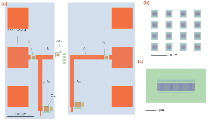
tools/em/ch18_pa/ch18_layout.py. (a) The Chapter 17 amplifier: GSG pads (bondpad cell), cap_rfcmim cells, 16 µm TopMetal2 lines (orange) over a Metal1 ground plane (light blue); the core (Rst, Cst, four npn13G2 cells) is placed but not wired. (b) The input device of the Chapter 9 LNA as 16 rfnmos cells (W = 8 µm, 4 fingers, L = 0.13 µm). (c) One npn13G2 cell with Nx = 4 (emitters 0.07 µm × 0.9 µm).MOSFETs: fingers, cells and the wiring between them
Chapter 6 showed how a wide RF MOSFET is drawn: many narrow fingers that share source and drain diffusions, contacted at both ends of the gate, grouped into cells, and that SG13G2’s RF model (rfmode=1) adds a fixed gate resistance RGO = 40 Ω per cell (Eq. 6.6) [205]. The fixed term stands for the gate ring and the contacts of one cell, so it divides by the number of cells, not by the number of fingers. The Chapter 9 LNA’s 128 µm input device is therefore drawn as \(m\) = 16 cells of four 2 µm fingers, which brings its model gate resistance to 3.36 Ω; as one cell of 64 fingers it would be above 40 Ω, and the LNA’s noise figure would be lost to it.
In the layout, \(m\) = 16 means sixteen instances of the PDK’s rfnmos cell (Figure 18.1b), each 4.28 µm × 4.88 µm with its own gate ring and guard ring, because that is the structure IHP measured to fit the RF model. What the model cannot know is how the cells are joined. Sixteen cells in a 4 × 4 array occupy about 31.3 µm × 25.9 µm, and the gate, drain and source buses that join them are interconnect the extraction or the EM simulation must add.
Worked example 18.1 · The gate bus of the LNA input device
Join the gates of the 16 cells with a Metal2 bus 2 µm wide that runs 30 µm across the array and is fed at one end. Metal2 is 0.49 µm thick with σ = 2.32 × 10⁷ S/m, a sheet resistance of 0.088 Ω/sq, so the bus is 15 squares, 1.32 Ω from end to end. The cells draw their gate current all along it, so, like the gate finger of Eq. (6.5), it acts as a third of its end-to-end resistance: 0.44 Ω, 13 % on top of the model’s 3.36 Ω. Fed from the centre instead, each half is 0.66 Ω and acts as a third of that in parallel with the other half: 0.11 Ω. The gate bus also has 0.308 pH/µm-class inductance and capacitance to the source bus beneath it, which adds to Cgs. Feed wide devices from the centre, or with a tree of equal branches, and route the drain bus away from the gate bus to keep Cgd small.
HBTs: emitters, heat and the ground connection
An SG13G2 HBT is drawn by the npn13G2 cell, whose emitters are narrow stripes, 0.07 µm × 0.9 µm, between base contacts, with the collector contacted outside the active area (Figure 18.1c: Nx = 4, 12.2 µm × 7.11 µm). The Chapter 17 stage uses four such cells in parallel rather than one cell with 16 emitters, for the same reason as the MOSFET’s cells: the model was fitted to the cell, and large Nx made the transient simulations fail.
Parallel bipolar transistors share their current only as long as they share their temperature. At constant VBE the collector current rises steeply with temperature, so a device that runs warmer, because it sits in the middle of the array or nearer a hot neighbour, takes more current, heats further and, in the worst case, takes all of it; in multi-finger power HBTs this ends in a collapse of the current gain [173]. A simple ngspice check with the PDK model, four Nx = 4 cells at 27.5 mA in total, VCE = 1.5 V and self-heating on, puts numbers on it: with one cell 10 K warmer than the others it carries 7.48 mA against 6.67 mA, 12 % more. One ohm of emitter ballast per cell only trims this to 11 %, and 20 Ω of base ballast changes nothing, because at β ≈ 466 it is worth 0.04 Ω in the emitter. These SiGe devices run at 27 mA/µm², where their own emitter and base resistances already ballast them; the layout’s job is to keep the temperatures equal: space the cells evenly, give them the same thermal surroundings, and keep the hot output stage away from temperature-sensitive circuits such as bias references.
The emitter connection matters more at 50 GHz. Each cell’s emitter must reach the ground plane through the shortest via stack possible, because 3 pH of common emitter inductance, 10 µm of wire by Eq. (18.1), costs about a decibel of gain (Section 17.6). In Figure 18.1a the transistors therefore sit in a window of the ground plane between the two networks, with the base line arriving from one side, the collector line leaving from the other and the emitters strapped to the plane on both sides.
18.3 Laying out passives
Inductors and their keep-outs
The PDK’s inductor2 and inductor3 cells draw symmetric octagonal spirals of two and three terminals on TopMetal2, like the spirals of Chapter 7 [191]. Beside the metal, each cell draws a set of marker layers that tell the rest of the flow how to treat it: nofill layers on every metal and on Activ and GatPoly, so that the automatic fill keeps out of the field; a PWell block, which leaves the lightly doped substrate under the spiral and so lowers its eddy-current loss; and an NoRCX marker, which tells parasitic extraction to skip the spiral because an EM model describes it. Keep everything else out of the same area, and place substrate contacts or a guard ring around it at about the spiral’s radius: closer, and the ring carries induced currents that lower the Q (Chapter 7’s ground frame sat half a diameter away). The spirals the course uses are the EM-fitted models of Chapter 7 (tools/figs/_ch07_inductor.py); Chapter 7 explains how they were drawn and simulated, and that work is not repeated here.
MIM capacitors
The rfcmim cell (Figure 18.1a) draws exactly what the cap_rfcmim model of Chapter 7 describes: the MIM plate over a Metal5 bottom plate, an array of Vmim vias to the TopMetal1 top-plate connection, a feed of width wfeed on each side (TopMetal1 on one, Metal5 on the other) and a ring of substrate contacts (Activ, contacts and Metal1) around the bottom plate, which the model’s substrate network assumes. Two layout choices change the capacitor’s quality:
- The feed width is a model parameter. Chapter 7 found that a 30 µm capacitor with the default 2 µm feed has Q = 35.6 at 4.88 GHz, and 87.3 with a 10 µm feed. Draw the cell with the wfeed you simulated.
- The connection to the lines is not part of the model. A TopMetal2 line reaches the top plate through a landing of TopVia2 vias onto TopMetal1, and the bottom plate through Metal5, TopVia1, TopMetal1 and TopVia2. Each landing in Figure 18.1a is 8 µm × 16 µm, a few picohenries by Eq. (18.1), and it moves the capacitor’s apparent value at 50 GHz, where a 10 µm cap_rfcmim is only −j16.7 Ω.
A decoupling capacitor shorts its node to ground only if its ground plate reaches the plane: the 20 µm capacitors at the ends of the two stubs have their Metal5 plates tied to Metal1 through a stack of Via4 to Via1 right next to the cell.
Lines and the ground plane
The lines of Chapter 17 are 16 µm TopMetal2 microstrips over Metal1. In the layout they meet at T-junctions, where the stubs branch, and at the landings of the capacitors; these discontinuities have no line model and are what the EM simulation of Section 18.5 adds. The ground plane itself must obey the design rules [210]: SG13G2 requires slits in any metal wider than 30 µm (rule Slt.c), drawn on the metal’s slit purpose, at most 20 µm long, with enclosures and spacings to vias. The layout script places them on a staggered grid and keeps them away from the lines, where they would cut the return current; Section 18.6 reports what remains.
Common pitfall · Drawing a ground plane that the rules forbid
A solid sheet of Metal1 under a 450 µm amplifier, the natural ground for an EM simulation, fails the slit rule at once, and a whole chip of it fails the density rules (maximum metal density per window). Slits that run along the current, as in our ground plane, hardly change a microstrip, but slits across it, or a meshed plane with large holes, raise the line’s inductance and loss. Draw the slits early, and if they are large or cross a line, simulate them: gds2palace reads only the drawing purpose of each layer, so slits drawn on the slit purpose are invisible to the EM model, as they were in our runs.
18.4 Pads, probes and ESD
GSG pads and their capacitance
A millimetre-wave chip is measured on a probe station with ground–signal–ground (GSG) probes: three tips at a pitch of 100 or 150 µm that land on a row of three pads, the signal pad between two ground pads. The ground pads are tied to the chip’s ground plane through the full metal stack; the signal pad is the circuit’s input or output, and its capacitance to the ground below it is part of the matching network. Chapters 9 and 17 assumed 30 fF, a parallel-plate estimate with some fringing for an 80 µm TopMetal2 pad over a Metal1 shield:
Key equation · Pad capacitance
\[C_{pad} \approx \frac{\varepsilon_0\varepsilon_r A}{h} + C_{fringe}. \tag{18.2}\]
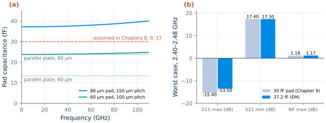
With \(A\) = 80 µm × 80 µm, \(h\) = 9.77 µm from the bottom of TopMetal2 to the top of Metal1 and \(\varepsilon_r\) = 4.1, the parallel-plate term is 23.8 fF. We simulated two GSG groups with Palace, each a TopMetal2-only signal pad (the PDK’s bondpad cell without its metal stack) over a solid Metal1 shield that extends under the whole group, ground pads stacked down to Metal1, and one port from the shield up to the centre of the signal pad, where a probe lands (Table 18.1, Figure 18.2a).
Table 18.1. Pad capacitance: EM (Palace, second-order elements) against the parallel-plate term of Eq. (18.2).
| Signal pad (GSG pitch) | Parallel plate | EM at 2.44 GHz | EM at 50 GHz | Fringing |
|---|---|---|---|---|
| 80 µm square, TopMetal2 (150 µm) | 23.8 fF | 37.2 fF | 37.7 fF | +56.3 % |
| 60 µm square, TopMetal2 (100 µm) | 13.4 fF | 23.8 fF | 24 fF | +77.6 % |
| PDK default bondpad: 80 µm octagon, Metal3–TopMetal2 stack | 123 fF (Metal3 to Metal1, by hand) | – | – | – |
The 80 µm pad has 37.2 fF, a quarter more than assumed. The fringing field, from the pad’s edges to the shield beyond them and to the ground pads, adds 56.3 % to the parallel-plate value, more than the 6 fF the earlier estimate allowed. The capacitance rises slowly with frequency, to 37.7 fF at 50 GHz, as the inductance of the pad and of the port’s vertical path starts to resonate with it. A 60 µm pad, which a 100 µm-pitch probe needs anyway, has 23.8 fF, 36 % less. The PDK’s default bondpad cell is a different object: it stacks Metal3 to TopMetal2 for wire bonding, and its Metal3 plate is only 1.57 µm above a Metal1 shield, so its parallel-plate term alone is about 123 fF (without a shield it couples to the lossy substrate instead). For RF signals, use a top-metal pad over a shield, as small as the probe or bond allows.
sp, tt, 27 °C.What the real pad does to Chapters 9 and 17
In the Chapter 9 LNA the pad is in parallel with the 54.7 fF of the ESD diodes, so the input node sees 91.9 fF instead of 84.7 fF. Re-simulating the final design of Chapter 9 with nothing else changed (Figure 18.2b) moves the input match: S11 at 2.44 GHz rises from −21 to −17.3 dB and its worst case in the band from −15.4 to −13.5 dB, still within the −10 dB specification; the −10 dB band shifts down from 2.23–2.61 GHz to 2.21–2.57 GHz. The gain falls by 0.1 dB and the noise figure does not change (1.17 dB at worst). At 2.4 GHz the extra 7 fF is a reactance of 9.1 kΩ; the LNA keeps every specification, and a small trim of Lg would re-centre its match.
In the Chapter 17 amplifier the pad sits directly in the output network, and it limits the load the collector can see. A series element behind a pad that is loaded by 50 Ω can only present resistances down to
\[R_{min} = \mathrm{Re}\left(R_0 \parallel \frac{1}{j\omega C_{pad}}\right) = \frac{R_0}{1 + (\omega C_{pad} R_0)^2}, \tag{18.3}\]40.9 Ω with 30 fF and 37 Ω with the EM’s 37.7 fF: the load-line value of 45 Ω remains reachable. Replacing 30 fF by 37.7 fF in Chapter 17’s own circuit, with its line lengths unchanged, lowers S21 at 50 GHz from 9.07 to 9.02 dB, raises S11 to −22.9 dB and S22 to −8.77 dB; re-solving the four line lengths for Eq. (17.2) restores the input match and gives 8.94 dB and S22 = −9.21 dB. On its own, the pad is a small correction; Section 18.6 shows that the rest of the layout is not.
ESD protection at radio frequencies
Every pad that leaves the chip needs a path for electrostatic discharge. The Chapter 9 LNA uses SG13G2’s 2 kV diodes to VDD and ground, which add 54.7 fF: at 2.4 GHz that is part of the match and costs little. At 50 GHz the same diodes would be −j58 Ω, more than the pad itself, and lossy. Millimetre-wave circuits therefore protect their pads with the matching network: a shunt stub to ground (or to a supply with a clamp) is a short for the slow discharge pulse and, at its design frequency, part of the match or, a quarter-wavelength long, invisible. The Chapter 17 amplifier does not yet have this: both of its pads are DC-blocked by a MIM capacitor, so a discharge into the input pad would cross the thin MIM dielectric. A version for tape-out adds a shunt stub to ground at each pad (and re-solves the match with it), or small diodes that the EM and the match include.
18.5 Electromagnetic extraction and co-simulation
The flow
The EM simulations of this chapter use Palace, AWS’s open-source finite-element solver for Maxwell’s equations [197], through IHP’s gds2palace workflow, as Chapter 7 did [198, 206] (Figure 18.3):
- Layout.
tools/em/ch18_pa/ch18_layout.pydraws each structure with KLayout’s Python API [203] and the PDK’s pcells, and marks each port as a thin box on layer 200 + n. - Stack-up. Because every structure sits over a solid Metal1 plane, we use IHP’s stack-up without the silicon substrate (
SG13G2_nosub.xml), as Chapter 7 did for its lines: the plane shields the substrate, and the model gets smaller. - Ports. Each port is a vertical 50 Ω lumped port from Metal1 up to TopMetal2: at the centre of a signal pad (the probe tip), and at the cut planes where the networks meet the circuit: the transistor’s base and collector side, the bias resistor and the supply.
- Mesh and solve. gds2palace models each metal as an impedance sheet of its real thickness and conductivity, meshes the volume with gmsh, and Palace runs an adaptive frequency sweep: it solves the full problem at a few frequencies and builds a reduced-order model from them.
- Back to the circuit. The S-parameters go into a Python cascade with the transistor’s simulated S-parameters, and into ngspice as a vector-fitted subcircuit.
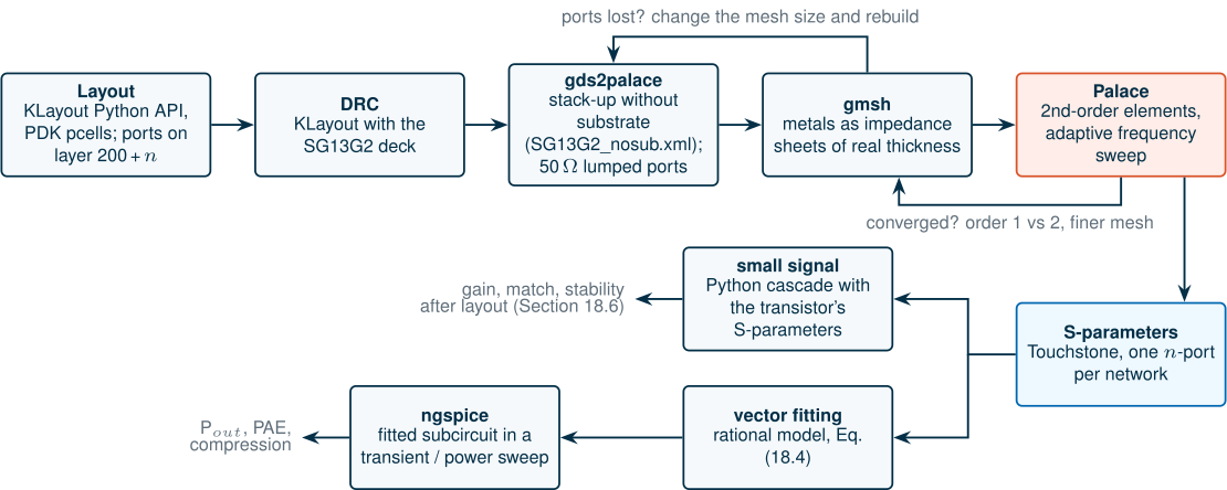
Two practical problems appeared. First, gmsh’s geometry operations are fragile: for some combinations of mesh size and air margin the model silently lost its port surfaces (and with them its excitations), so ch18_palace.py checks the generated configuration and rebuilds with a slightly different mesh size until every port is present. Second, and more important, the order of the finite elements.
Is it converged?
Chapter 2 ran its line with first-order elements because the second-order run did not finish. First-order elements are about five times cheaper for the same mesh, so we first simulated the amplifier’s networks with them. To judge the result, we ran Chapter 7’s 300 µm TopMetal2 line again with first-order elements on the same 4 µm mesh, and with second-order elements on a coarser 6 µm mesh, and compared both with Chapter 7’s second-order, 4 µm result (Table 18.2).
Table 18.2. The 300 µm TopMetal2 line of Chapter 7 at 50 GHz with three discretizations (Zc and βℓ from the line's ABCD matrix, port parasitics included).
| Elements, mesh on conductors | Zc | βℓ | Loss | Unknowns |
|---|---|---|---|---|
| 2nd order, 4 µm (Chapter 7) | 48.3 Ω | 36.2° | 0.604 dB/mm | 121 782 |
| 2nd order, 6 µm | 47.7 Ω | 36.3° | 0.616 dB/mm | 78 212 |
| 1st order, 4 µm | 41.4 Ω | 38° | 0.704 dB/mm | 23 533 |
The first-order line is 14 % low in impedance, 5 % long and 17 % lossier: its mesh of linear elements cannot represent the field between the strip and the plane, 9.8 µm below, with a few elements. The second-order result on the coarser mesh agrees with the reference within 1.2 % in Zc and 2 % in loss. A matching network built of such lines inherits the error: with first-order networks, the amplifier’s gain at 50 GHz came out 2.96 dB, and with second-order ones 4.82 dB. Every network result below therefore uses second-order elements, on a 6 µm mesh for the input network and a 7 µm mesh for the output network, whose 6 µm model lost its ports in gmsh; by Table 18.2 the coarser mesh costs about a percent in Zc.
Common pitfall · Trusting an EM result because it ran
An EM solver always returns S-parameters. Whether they are right depends on the mesh and the element order, and the only way to know is to change them and see whether the answer moves. Check a simple structure whose answer you know, such as a line against a two-line extraction or a closed-form Z0, with the settings you intend to use, before you trust a complex one.
The price of the second-order runs on a laptop shared with other jobs is in Table 18.3. The pads, with one port each, take 2.3 and 17 minutes; the networks, with three ports each and a sweep to 160 GHz, about 220 and 51 minutes (the first while another EM job shared the machine).
Table 18.3. Cost of the Palace runs (second-order elements, adaptive sweep, IIC-OSIC-TOOLS in Docker on a laptop, other jobs running).
| Structure | Ports | Unknowns | Samples | Processes | Time | Peak memory |
|---|---|---|---|---|---|---|
| GSG pad, 60 µm | 1 | 213 280 | 4 | 2 | 2.3 min | 1.9 GB |
| GSG pad, 80 µm | 1 | 352 892 | 4 | 2 | 17 min | 3.1 GB |
| Input network (pad, Ci, ℓi, ℓsi, Cdec), 6 µm mesh | 3 | 384 862 | 15 | 3 | 220 min | 4.4 GB |
| Output network (ℓso, Cdec, ℓo, Co, pad), 7 µm mesh | 3 | 338 518 | 17 | 3 | 51 min | 3.7 GB |
Bringing the result into ngspice
A Python cascade of S-parameters is exact for small signals, but a power sweep needs the networks inside a transient simulation. ngspice cannot read a Touchstone file, so the EM S-parameters are first approximated by a rational function with vector fitting [172]:
Key equation · A rational model of an EM n-port
\[\mathbf{S}(s) \approx \mathbf{D} + \sum_{k} \frac{\mathbf{R}_k}{s - p_k}. \tag{18.4}\]
All elements of the 3 × 3 matrix share one set of stable poles \(p_k\) (real, or complex pairs), which the algorithm relocates over a few linear least-squares iterations; then the residue matrices \(\mathbf{R}_k\) and the constant \(\mathbf{D}\) are fitted with the poles fixed. Each pole becomes a small RC state in the netlist, and each port a resistor \(Z_0\) in series with a controlled source that sets the reflected wave:
\[V_i = Z_0 I_i + 2b_i, \qquad a_i = V_i - b_i, \qquad \mathbf{b} = \mathbf{S}\,\mathbf{a}. \tag{18.5}\]Derivation · The circuit of a fitted S-matrix
With the reference impedance \(Z_0\) and the port current \(I_i\) flowing into the network, the incident and reflected waves, in volts, are \(a_i = (V_i + Z_0I_i)/2\) and \(b_i = (V_i - Z_0I_i)/2\). Subtracting gives \(V_i = Z_0I_i + 2b_i\): the port is a resistor \(Z_0\) in series with a voltage source \(2b_i\). Adding gives \(a_i = V_i - b_i\), which a behavioural source computes from the port node and the internal node. For each pole, the state \(x = a_j/(s - p)\) obeys \(\dot x = p\,x + a_j\); on a node with a capacitor \(C_0\) to ground this is a conductance \(-C_0p\) in parallel and a current source \(C_0a_j\), scaled by \(\omega_0\) so that the node voltage is of the order of the port voltages. A complex pair \(p = \sigma + j\omega\) needs two such nodes, \(x_1 + jx_2\), coupled by currents \(\mp C_0\omega x\). The reflected wave is then \(b_i = \sum_j D_{ij}a_j + \sum_{j,k} R_{k,ij}\,x_{jk}\), a linear behavioural source. The realization uses only capacitors, resistors and linear controlled sources, so it works in ngspice’s op, ac, sp and tran.
tools/figs/_ch18_vf.py implements both steps. For the two networks, 5 and 7 complex pole pairs plus two real poles fit the EM data from 0.01 to 160 GHz with an rms error of 0.000197 and 0.000109, and an ngspice sp of each subcircuit alone reproduces the EM S-parameters within 0.0006 from 10 to 160 GHz. A fitted model must also be passive: no singular value of its S-matrix may exceed one, at any frequency, or a transient simulation can oscillate. Our fits stay below 1.002 up to 1 THz; where a fit exceeds one by a fraction of a percent above its band, the script scales it down by that fraction.
18.6 Verifying an RF block: the 50 GHz amplifier
Chapter 17 designed a one-stage SiGe amplifier for 50 GHz and ended without an EM simulation, with 9.07 dB of gain against a 10 dB target and S22 = −9.47 dB. This section lays its matching networks out, checks them against the design rules, simulates them with Palace and puts the result back into Chapter 17’s circuit, without changing anything else: the same transistor (four npn13G2 with Nx = 4 at 27.5 mA), the same stabilizing Rst ∥ Cst, bias resistor and supply.
The layout
Figure 18.1a shows the result, 498 µm × 445 µm including the pads. Each network is drawn as Chapter 17’s circuit (Figure 17.1) with its line lengths of Section 17.4, measured from the centre of each T-junction: on the input, the GSG pad, the 10 µm DC block Ci, the junction, the series line ℓi = 48.6 µm towards the base and the stub ℓsi = 197 µm down to the 20 µm decoupling capacitor, from which a 4 µm feed leads to RB; on the output, the stub ℓso = 181 µm from the collector to its decoupling capacitor and an 8 µm supply feed, the series line ℓo = 115 µm, the DC block Co and the pad. Every capacitor is the PDK’s rfcmim cell with the 2 µm feed of the model Chapter 17 simulated; every line is the 16 µm TopMetal2 microstrip; a Metal1 plane lies under all of it. The EM ports sit at the pad centres (where the probes land), at the ends of ℓi and of the collector junction (the cut planes towards the transistor), and at the ends of the bias and supply feeds.
Design-rule check
The PDK’s KLayout rule deck [210] checks each network in about 20 s (maximum rule set, density rules off, because fill is added at chip level). The first run found only slit violations: the Metal1 plane, and the TopMetal2 signal pads, which we had drawn with the bondpad cell’s probe-pad option that omits the dfpad marker the rules use to recognize a pad. With the pads marked and the plane slitted (Section 18.3), the GSG pad group passes with no violations. Each network keeps two small regions of the plane that rule Slt.c still flags, around the decoupling capacitor at the end of the stub and around the landings of the DC block, where the keep-outs around lines, vias and capacitor cells leave no room for a 3 µm slit, and one or two instances of the recommended rule Pad.d1R: the substrate-contact ring of the capacitor cells is 10.1 µm from the pad opening instead of 11.2 µm. Neither changes the EM model, and both would be fixed by hand (slits along the current under the landings, 2 µm more feed between pad and capacitor) before tape-out. The core is placed but not wired, so LVS and antenna checks were not run.
What the EM simulation finds
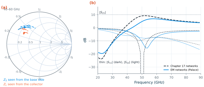
Figure 18.4 and Table 18.4 put the two EM networks into Chapter 17’s amplifier in place of its line-and-capacitor networks. The result is not a small correction. At 50 GHz the gain falls from 9.07 dB to 4.82 dB, S11 rises from −62.9 to −10.8 dB and S22 from −9.47 to −7.79 dB. The gain peak moves from 52.5 GHz (9.22 dB) to 57.5 GHz and drops to 6.87 dB. Each network on its own costs about 2 dB: with only the input network from EM the gain is 6.8 dB, with only the output network 7.14 dB.
Three differences between the schematic networks and the drawn ones explain it.
- More capacitance and more inductance. At 1 GHz the pad port of the input network sees 208 fF instead of 182 fF: 7 fF of it is the larger pad (Section 18.4), the rest is the DC block’s fringing and the landings. The stubs, through their landings and the via stacks of the decoupling capacitors, are 246 pH instead of 220 pH on the input and 215 pH instead of 162 pH on the output. At 50 GHz, where the networks have the Q of 5 to 6 that Section 17.4 found, these shifts move both impedances: the source impedance seen from the base side becomes 11.2 + j22.2 Ω instead of 13.8 + j27.5 Ω, and the collector sees a parallel resistance of 31.2 Ω instead of the 45 Ω the load line asked for (Figure 18.4a).
- More loss. Driven at its pad with 50 Ω on the other ports, the input network dissipates 28.9 % of the power at 50 GHz, against 15.4 % for the schematic network, and the output network 38.1 % against 22.9 %. In the amplifier, the input network delivers 36.9 % of its input power to the transistor (Chapter 17: 55.7 %), and the output network 48.3 % of the collector power to the load (79.8 %). The extra loss is in what the schematic did not have: the landings, the narrow capacitor feeds, the thin Metal5 plates and the return current in the Metal1 plane around them. By Eq. (17.3), a network of loaded Q 5 to 6 turns every bit of extra series resistance into a large loss.
- The emitter. The networks end at the transistor’s cut planes; the emitter connection is not in them. With Chapter 17’s 3 pH of emitter inductance added, the gain falls further to 3.96 dB.
Can a lumped model explain the EM result well enough to re-solve the design with it? We fitted Chapter 17’s networks, with a pad capacitance, series inductances at both terminals of each DC block, line-length corrections and inductances in the stubs as free parameters, to the EM three-ports from 20 to 100 GHz. The fit reduces the rms error in S from 0.0744 to 0.0335 (input) and 0.0311 (output), but only with unphysical values: inductances of 53.5 and −42.2 pH on the two sides of Ci, −109 and 104 pH around Co. The differences are distributed through the layout, not concentrated in a few lumped parasitics, so the line lengths re-solved with such a model would mean nothing, and we do not use them. The way to retune this layout is to keep the EM in the loop: change the drawn lengths, re-simulate, and repeat. The gain peak of 6.87 dB at 57.5 GHz shows roughly what retuning the same networks to 50 GHz can recover: about 2 dB, not the 5.2 dB the target needs.
Large signal with the EM networks
For the power sweep, the two EM networks enter ngspice as the vector-fitted subcircuits of Section 18.5. An ngspice sp of the complete amplifier with them agrees with the Python cascade within 0.17 dB from 30 to 70 GHz (Figure 18.5a), and the amplifier stays unconditionally stable (μ ≥ 1) from 0.1 to 160 GHz, the band of the EM data. The bias point draws 26.4 mA instead of 27.5 mA, because the fitted subcircuits reproduce the networks’ DC resistance only approximately.
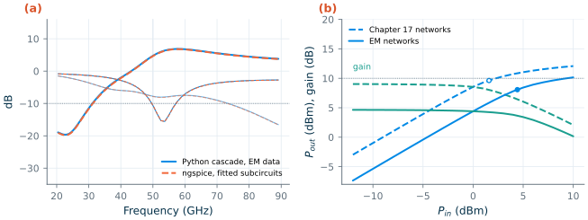
sp with the vector-fitted subcircuits (orange, dashed). (b) Pout (blue) and gain (teal) at 50 GHz against available input power, with Chapter 17's networks (dashed, Chapter 17's own result) and with the EM networks (solid); circles: P1dB. ngspice transient + FFT, 60 periods, as in Chapter 17.The transient power sweep (Figure 18.5b) starts from 4.64 dB of gain (Chapter 17: 9.03 dB), compresses by 1 dB at 8.07 dBm of output for 4.42 dBm of input (9.62 dBm), and reaches 10.2 dBm at +10 dBm of input (12.1 dBm). The PAE peaks at 7.44 % at 8.42 dBm (17.5 %), and at +10 dBm of output it is down to 2.18 %, because the input power is no longer small next to the output power. The collector peak falls from 3.12 to 2.84 V, since the collector sees a lower resistance.
Table 18.4. The 50 GHz amplifier of Chapter 17 against its target, before and after layout (typical models, 27 °C, VCC = 1.5 V; Chapter 17: TopMetal2 lines and cap_rfcmim; after layout: Palace networks of Figure 18.1a, order 2).
| Item | Target | Chapter 17 | After layout (EM) |
|---|---|---|---|
| Small-signal gain at 50 GHz | ≥ 10 dB | 9.07 dB ✗ | 4.82 dB ✗ |
| Gain peak | – | 9.22 dB at 52.5 GHz | 6.87 dB at 57.5 GHz |
| S11 at 50 GHz | ≤ −10 dB | −62.9 dB ✓ | −10.8 dB ✓ (marginal) |
| S22 at 50 GHz | ≤ −10 dB | −9.47 dB ✗ | −7.79 dB ✗ |
| Stability | μ > 1 | ✓ (0.1–400 GHz) | ✓ (0.1–160 GHz, the EM band) |
| P1dB (output) | ≈ +10 dBm | 9.62 dBm ✓ | 8.07 dBm ✗ |
| Psat | ≥ +10 dBm | 12.1 dBm ✓ | 10.2 dBm ✓ (marginal) |
| Peak PAE | (reported) | 17.5 % | 7.44 % |
The amplifier does not meet its target after layout. It misses the gain target by 5.2 dB instead of 0.9 dB, its output match by 2.2 dB, and it reaches +10 dBm only at full drive. Nothing in the transistor changed: the layout’s networks, built of the same lines and capacitors, are lossier and resonate elsewhere, and in a stage that already spent its gain margin on stability, that is decisive. The remedies of Section 17.7 become necessary rather than optional: a cascode or a second stage for gain, and networks with fewer transformations and wider feeds for loss; and the design loop must include the EM from the first layout, as the academy module does. Section 17.8 does exactly that: a cascode whose networks are designed on EM-simulated blocks (a DC block with its landings, a T-junction, a stub-end capacitor) keeps 12.4 dB of gain, S11 = −14.0 dB and S22 = −30.6 dB after layout and a full Palace check, with Psat = 11.4 dBm; only its P1dB, 7.95 dBm, stays short.
What this means for your design
At millimetre waves, simulate the layout of the passives before you believe the schematic. Our networks were drawn exactly to the schematic’s line lengths, with PDK cells, and still lost 4.3 dB. Lay out early, extract with EM at converged settings, check the order of the elements on a simple line, and plan for several EM iterations, not one.
18.7 Measurement and de-embedding
A layout that passes DRC and EM is ready to be measured. On a probe station, a vector network analyser is connected through cables and GSG probes, and calibrated on a substrate of known standards (short, open, load and thru, or the LRRM set), which moves the reference plane of the measurement to the probe tips. What lies between the tips and the circuit, the pads and their feeds, is then still part of the measurement, and there are two ways to deal with it.
Keep the pads in the design. The networks of Section 18.6 include their pads, with the EM ports where the probes land. The simulated S-parameters of the amplifier are therefore directly comparable with a calibrated measurement, and nothing has to be removed. This is the natural choice for a circuit that will be used with its pads, such as an amplifier that is bonded or probed in its application.
Remove the pads to see the device. To characterize a transistor or a spiral, the pads must be taken off the measurement. Chapter 3 derived open–short de-embedding [51], which treats the pads as a shunt admittance and the feeds as a series impedance, and showed its residual error at millimetre waves, where the feeds are distributed. Three remedies follow from this chapter. Better dummies, as in three-step de-embedding with an extra thru [52, 53]; short feeds, so that the lumped picture holds; or EM-based de-embedding: simulate the pad-and-feed structure alone, as we did for the 80 µm GSG group, and remove it as a two-port by multiplying the measurement with the inverse of its transmission matrix. The EM model of the pad is also a check of the measurement: an open pad that measures 30 fF where the EM says 37.2 fF points to a problem with the calibration or with the model.
A test chip for the amplifier of Chapter 17 would therefore carry, next to the amplifier: an open and a short of the pad-and-feed structure, a thru, and two TopMetal2 lines of different lengths for the two-line extraction of Eq. (7.12), which checks the line model that the whole match rests on. The measurement plan follows from the specification: S-parameters from 0.1 to 67 GHz or beyond (stability needs the low frequencies as well as the band), a power sweep at 50 GHz with a calibrated power sensor for P1dB, Psat and PAE, and the DC current at every step, which is also the first check of the bias network.
What this means for your design
Decide early where the reference plane is: at the probe tips (pads in the EM, nothing to de-embed) or at the device (pads and feeds out, with dummies on the chip). Put the dummies on the same chip, next to the circuit, and simulate them with the same EM settings as the circuit, so that measurement, de-embedding and simulation describe the same structure.
Try it · The layout and EM scripts
The layouts come from
tools/em/ch18_pa/ch18_layout.pyand the EM runs fromtools/em/ch18_pa/ch18_palace.py(both inside IIC-OSIC-TOOLS); every number of the chapter comes fromtools/figs/ch18_rf_layout.py, which redraws everything in a minute from the Touchstone files and the cached simulations intools/_work/ch18/(--rerunrepeats a part’s ngspice runs). Three experiments: (1) Runch18_palace.py TL300 --order 1 --cell 2 --tag _o1c2: does a finer first-order mesh approach the second-order line of Table 18.2, and at what cost in unknowns? (2) Inch18_layout.py, draw the input network with the 60 µm pad (pa_in(pad=60.0, pitch=100.0)), runch18_palace.py PAIN --cell 6and partem: how much of the input network’s loss and detuning was the pad’s? (3) In_ch18_vf.vectfit_s, restrictpairsto(3,)and rerun partspice --rerun: watch the ngspice result leave the Python cascade, and the largest singular value of the fit.
- At 50 GHz every wire is a component: a 16 µm TopMetal2 microstrip has 0.308 pH/µm and 0.135 fF/µm (Eq. 18.1), so 10 µm of emitter lead costs about a decibel. Give every RF signal a ground plane beneath it, keep high-current loops and emitter connections short, and draw the slits the rules require.
- Build RF MOSFETs from many cells (SG13G2’s model adds 40 Ω of gate resistance per cell) and join them with centre-fed buses; build HBTs from parallel cells at equal temperatures, because a cell 10 K warmer takes 12 % more current.
- An 80 µm TopMetal2 pad over a Metal1 shield has 37.2 fF, not 30 fF: fringing adds 56.3 % to the parallel plate. The Chapter 9 LNA keeps its specification (S11 ≤ −13.5 dB); a 60 µm pad has 23.8 fF, and the PDK’s stacked bond pad several times more.
- Palace through gds2palace extracts a layout’s passives, but only at converged settings: first-order elements made a line 14 % low in Zc and 17 % lossier. Vector fitting brings the S-parameters into ngspice for sp and transient analyses.
- After layout and EM, the Chapter 17 amplifier has 4.82 dB of gain instead of 9.07 dB, S22 = −7.79 dB, P1dB = 8.07 dBm, Psat = 10.2 dBm and 7.44 % peak PAE: it misses its 10 dB target by 5.2 dB, and a lumped fit cannot retune it; the EM belongs in the design loop.
- Keep the pads in the EM model and the simulation compares directly with a calibrated probe measurement; to see a device, de-embed the pads with on-chip dummies or with their own EM model.
Further reading
- S. P. Voinigescu, High-Frequency Integrated Circuits [10]: layout of SiGe HBTs and MOSFETs for millimetre waves, transmission-line interconnect, pads and the design-for-measurement of test structures.
- A. M. Niknejad, Electromagnetics for High-Speed Analog and Digital Communication Circuits [14]: the physics behind return paths, substrate coupling and on-chip lines.
- A. Hastings, The Art of Analog Layout [23]: matching, guard rings, substrate contacts and the general craft of analog layout, much of which applies unchanged at RF.
- W. Liu et al. [173]: thermal coupling and current-gain collapse in multi-finger power HBTs, the reason for even temperatures and ballasting.
- IHP’s Palace and openEMS workflows [198, 206, 197] and the SG13G2 DRC decks [210]: the tools of this chapter, with examples that include the core of the IHP Analog Academy’s 50 GHz amplifier [3].
- B. Gustavsen and A. Semlyen [172]: vector fitting, the method that turns EM S-parameters into a circuit.
- M. C. A. M. Koolen et al. [51] and E. P. Vandamme et al. [53]: de-embedding the pads of on-wafer measurements, from the open–short method to the improved three-step method.