Lab 1
Lines, the Smith Chart, Matching and De-embedding
Build an on-chip transmission line from electromagnetic data, match two loads with it and with lumped elements on the Smith chart, and remove a pair of probe pads from a transistor measurement, with scikit-rf doing the network algebra and ngspice checking the result.
- Extract the propagation constant and characteristic impedance of a line from two EM simulations, and use them as a scikit-rf medium.
- Compare an EM line with a closed-form microstrip model and say where the closed form fails on chip.
- Design an L-section and a single-stub match on the Smith chart with scikit-rf, and verify both in ngspice.
- Explain why a lossy line needs a complex characteristic impedance.
- De-embed a two-port with scikit-rf’s
OpenandOpenShortand reproduce Chapter 3’s Table 3.4.
Contents
| Lab 1 at a glance | |
|---|---|
| Goal | A TopMetal2 microstrip as a scikit-rf medium, two matching networks designed on the Smith chart and checked in ngspice, and open–short de-embedding against Chapter 3. |
| Chapters | Chapter 3 (Sections 3.1, 3.3, 3.4 and 3.8, Eq. 3.26, Table 3.4), Chapter 7 (Section 7.7, Eq. 7.12) and Chapter 8 (Sections 8.2, 8.4 and 8.6, Eqs. 8.3–8.4) |
| Time | 3 hours (the course plan splits it: lines and de-embedding after Chapter 3, matching after Chapter 8) |
| Files | tools/labs/lab1/: tline.py; matching.py, lmatch.cir, stub.cir; deembed.py, bare.cir, pads.cir, open.cir, short.cir, pads.inc. Chapter 7’s EM lines: tools/em/ch07_inductors/TL300.s2p, TL900.s2p |
| Run time | each script 2–3 s |
Run every command in tools/labs/lab1, inside the container or from your computer with ../common/iic.sh in front of it (Lab 0).
Hand calculation
- The L-section. The course PA wants \(R_{opt}\) = 10.6 Ω and the antenna is 50 Ω (Chapter 8, Worked example 8.1). With Eq. (8.3) find \(Q\), the series inductance on the 10.6 Ω side and the shunt capacitance on the 50 Ω side at 2.44 GHz. Estimate the −10 dB bandwidth with Eq. (8.4).
- The line at 50 GHz. Chapter 7’s 16 µm TopMetal2 microstrip has \(\varepsilon_{eff}\) = 3.73 at 50 GHz. What are the wavelength and a quarter-wavelength on it? How many degrees is a 139 µm line?
- The pads. Each GSG pad of Chapter 3’s model (Figure 3.8) is \(C_p\) = 35 fF in series with \(R_p\) = 20 Ω; the pads are coupled by \(C_c\) = 2 fF and each device plane has \(C_d\) = 3 fF. Is \(R_p\) negligible at 2.44 GHz? Estimate how much capacitance the pads add at the gate, and, since \(f_T \approx g_m/2\pi C_{in}\), what \(f_T\) a raw measurement of the bare device (\(C_{in}\) = 58.2 fF, \(f_T\) = 45.8 GHz) would suggest.
Steps
A. The TopMetal2 line as a scikit-rf medium
- Run
python3 tline.py. It reads Chapter 7’s Palace results for 300 µm and 900 µm of the same line as scikit-rfNetworks and applies Eq. (7.12): the eigenvalues of \(\mathbf{T}_{900}\mathbf{T}_{300}^{-1}\) (the ABCD matrices,Network.a) are \(e^{\pm\gamma \cdot 600\,\mu\mathrm{m}}\), whatever the ports of the EM model added. From \(\gamma = \alpha + j\beta\) it prints the loss \(8.686\,\alpha\) in dB/mm and \(\varepsilon_{eff} = (c\beta/\omega)^2\), and \(Z_0 = \sqrt{B/C}\) from the long line. -
The script then builds the medium
tm2 = rf.media.DefinedGammaZ0(frequency=freq, z0_port=50, z0=z0, gamma=gamma)and checks it:
tm2.line(600, unit="um") ** tl300(600 µm of medium cascaded with the 300 µm EM line) must reproduce the 900 µm EM line.z0_port=50makes the line’s S-parameters refer to 50 Ω ports, like the EM files; without it they refer to the line’s own \(Z_0\), and the cascade compares different things. - Finally it asks scikit-rf’s closed-form microstrip,
media.MLine(Hammerstad–Jensen [105], with Kirschning–Jansen dispersion), for the same strip: \(w\) = 16 µm, \(h\) = 9.77 µm, \(t\) = 3 µm, \(\varepsilon_r\) = 4.1, TopMetal2’s resistivity. Its warning that the conductor-loss formula is invalid when the strip is thinner than three skin depths is real: below about 10 GHz the MLine loss is meaningless here. Figure L1.1 compares the two.
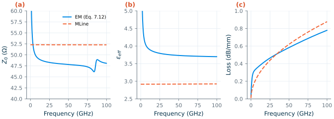
MLine for the same cross-section (orange, dashed). (a) Z0, (b) εeff, (c) loss.B. An L-section at 2.44 GHz
-
Run
python3 matching.py(it does parts B and C). Part B computes the L-section of your hand calculation and builds it from scikit-rf’s lumped elements:lump = rf.media.DefinedGammaZ0(frequency=freq, z0=50) lsec = lump.inductor(L) ** lump.shunt_capacitor(C) # port 1: PA side, port 2: antenna lsec.renormalize([10.6, 50]) # S-parameters between the real terminationsIt finds the −10 dB band of \(\vert S_{11}\vert\), writes the values into
out/lmatch.incand runslmatch.cir, the same network in ngspice with a 10.6 Ω port. Then it traces the match on the Smith chart, looking from the PA towards the antenna, as in Worked example 8.2: the shunt capacitor moves 50 Ω along the circle \(g\) = 1, the series inductor along a circle of constant \(r\) to 10.6 Ω (Figure L1.2a). Each arc is the same network evaluated at 2.44 GHz while the element grows from zero.
C. A single-stub match at 50 GHz
- Part C matches Chapter 8’s 50 GHz load, 20 Ω in series with 79.6 fF (\(z_L\) = 0.4 − j0.8), to 50 Ω with a line and a shorted stub on the TopMetal2 microstrip. The design uses Chapter 7’s constants at 50 GHz, read from part A (\(Z_0\) = 47.8 Ω, \(\varepsilon_{eff}\) = 3.73) and no loss. On the Smith chart, the line rotates the load on a circle of constant \(\vert\Gamma\vert\) until it reaches \(g\) = 1; the script finds that length with
scipy.optimize.brentqon the admittance oftl.line(d, "m") ** load, then the stub length whose admittance,tl.delay_short(l, "m"), cancels the remaining susceptance (Figure L1.2b). - The match is then evaluated, from 30 to 70 GHz, on four versions of the line: lossless; “naive”, with the 0.583 dB/mm loss added to a real 47.8 Ω;
media.DistributedCircuitwith \(R'\), \(L'\) and \(C'\) computed from the same \(Z_0\), \(\varepsilon_{eff}\) and loss; and the frequency-dependent EM medium of part A.stub.cirrepeats it in ngspice with LTRA lines and the same \(R'\), \(L'\), \(C'\), as Chapter 8 did (Figure L1.2c).
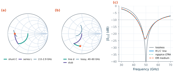
Common pitfall · A lossy line with a real Z0
Adding the attenuation to a lossless line, \(\gamma = \alpha + j\beta\) with a real \(Z_0\), looks harmless, but no physical line behaves like that: a series resistance \(R'\) also makes \(Z_0 = \sqrt{(R' + j\omega L')/(G' + j\omega C')}\) complex, here 47.8 − j1.58 Ω at 50 GHz. For the shorted stub, which carries a large standing wave, the difference matters: the naive line loses 0.456 dB, the consistent \(R'L'C'\) line 0.717 dB. Build lossy lines from \(R'\), \(L'\), \(G'\), \(C'\) (
media.DistributedCircuit) or from extracted \(\gamma\) and \(Z_0\) together, as in part A.
Common pitfall ·
meas ... whenafter anspanalysisIn ngspice-47 a
meas sp ... whenstatement (for example, the frequency where \(\vert S_{11}\vert\) crosses −10 dB) crashes ngspice with a segmentation fault;meas sp ... find ... at=works. The lab netlists therefore write the curves withwrdataandlabkit.band_edgesfinds the band edges in Python.
D. Open–short de-embedding
- Run
python3 deembed.py. It runs four netlists, each a separate two-portsprun from 97.1 MHz to 97.1 GHz, 40 points per decade, so that 2.44 GHz is one of the points:bare.cir, Chapter 3’s nMOS (20 fingers of 2/0.13 µm,rfmode=1, \(V_{DS}\) = 0.6 V) alone. Its control block sweeps \(V_{GS}\), measures the voltage for 2.00 mA, sets it withalter, and writes it intoout/bias.incwithecho;pads.cir, the same device between the pads and feeds ofpads.inc(the subcircuit of Figure 3.8b), biased with that voltage through bias tees outside the pads, as on a probe station;open.cirandshort.cir, the two dummies.
-
The script de-embeds the raw measurement with scikit-rf [215],
from skrf.calibration.deembedding import Open, OpenShort
dut = OpenShort(dummy_open=dut_open, dummy_short=dut_short).deembed(raw)
applies Eq. (3.26) by hand to the Y-matrices as a check, and prints Chapter 3’s Table 3.4 from its own runs: the input capacitance \(\mathrm{Im}(Y_{11})/\omega\) and resistance \(\mathrm{Re}(1/Y_{11})\) at 2.44 GHz, the errors of \(Y_{11}\) and \(Y_{21}\) against the bare device, \(f_T\) where \(\vert h_{21}\vert = \vert Y_{21}/Y_{11}\vert\) crosses one and \(f_{max}\) where scikit-rf’s
unilateral_gain(Mason’s U) does (Figure L1.3).
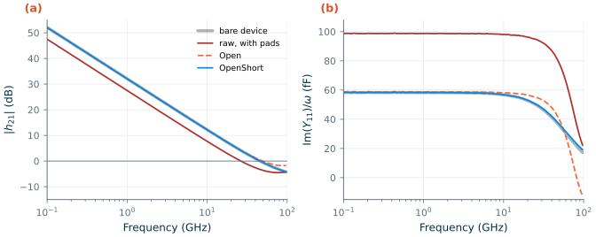
Open; blue: OpenShort. This is Chapter 3's Figure 3.9, redrawn from the lab's runs.Checkpoint
Table L1.1. Part A: the 16 µm TopMetal2 microstrip (tolerance ±1 in the last digit).
| Quantity | EM line (Eq. 7.12) | Chapter 7 | scikit-rf MLine |
|---|---|---|---|
| \(Z_0\) at 4.88 / 50 GHz | 50.7 / 47.8 Ω | 50.7 / 47.8 Ω | 52.3 / 52.3 Ω |
| \(\varepsilon_{eff}\) at 4.88 / 50 GHz | 4.16 / 3.73 | 4.16 / 3.73 | 2.92 / 2.92 |
| Loss at 2.44 / 4.88 / 50 GHz | 0.283 / 0.325 / 0.583 dB/mm | 0.283 / 0.325 / 0.583 dB/mm | 0.137 / 0.194 / 0.620 dB/mm |
| λ/4 at 50 GHz | 776 µm | 776 µm | |
Check: largest \(\vert S_{21}\vert\) error of line(600 µm) ** TL300 against TL900 |
0.0024 |
Table L1.2. Parts B and C: the two matches (scikit-rf unless marked ngspice; tolerance ±1 in the last digit, hand values ±1 %).
| Quantity | Lab 1 | Chapter 8 |
|---|---|---|
| L-section: \(Q\), \(L\), \(C\) (hand and script) | 1.928, 1.333 nH, 2.515 pF | 1.93, 1.33 nH, 2.52 pF |
| L-section: impedance after the shunt C, normalized | 0.212 − j0.409 | 0.212 − j0.409 |
| L-section: −10 dB band, scikit-rf / ngspice / Eq. (8.4) | 1.906–2.876 GHz = 39.7 % / 39.7 % / 34.6 % | 39.7 % (ideal elements) |
| Stub: line length \(d\), admittance there | 139.3 µm (16.2°), y = 1.000 + j1.611 | 139 µm (16.2°), 1.00 + j1.61 |
| Stub: shorted stub length | 284.6 µm (33.0°) | 285 µm (33.0°) |
| Lossless: −10 dB band | 33.6 % | |
| \(R'L'C'\) line: \(R'\), \(L'\), \(C'\) per mm | 6.42 Ω, 0.308 nH, 0.135 pF | 6.42 Ω, 0.308 nH, 0.135 pF |
\(R'L'C'\) line (DistributedCircuit): \(\vert S_{11}\vert\), loss, −10 dB band at 50 GHz |
−23.4 dB, 0.717 dB, 36.1 % | about −23 dB, 0.717 dB, 36.1 % |
ngspice, LTRA lines (stub.cir) |
−23.3 dB, 0.716 dB, 36.1 % | |
| EM medium of part A | −23.4 dB, 0.712 dB, 36.3 % | |
| Naive lossy line (real \(Z_0\)) | −26.9 dB, 0.456 dB, 34.9 % |
Table L1.3. Part D: the transistor of Chapter 3 seen through the pads, raw and de-embedded with scikit-rf (errors relative to the bare device; tolerance ±1 in the last digit). Every entry equals Chapter 3's Table 3.4.
| Bare device | Raw, with pads | Open |
OpenShort |
|
|---|---|---|---|---|
| Input capacitance at 2.44 GHz | 58.2 fF | 98.6 fF | 58.6 fF | 58.1 fF |
| Series input resistance at 2.44 GHz | 44.3 Ω | 17.3 Ω | 41.7 Ω | 44.5 Ω |
| Error of \(Y_{11}\) at 2.44 GHz | – | 69.5 % | 0.84 % | 0.055 % |
| Error of \(Y_{11}\) / \(Y_{21}\) at 50 GHz | – | 109 % / 60.5 % | 40.3 % / 56.3 % | 2.99 % / 3.08 % |
| \(f_T\) | 45.8 GHz | 26.4 GHz | 49.4 GHz | 45.9 GHz |
| \(f_{max}\) | 37.5 GHz | 32.7 GHz | 36.3 GHz | 37.4 GHz |
The drain current is 2.000 mA alone and 1.998 mA with the pads, at \(V_{GS}\) = 0.6998 V; scikit-rf’s OpenShort and Eq. (3.26) by hand agree to a relative 6 × 10⁻¹⁴. Every Chapter 7 and Chapter 8 value in the tables is reproduced; the “about −23 dB” is read from Chapter 8’s Figure 8.7c, whose script gives −23.4 dB. The hand estimates of part B are exact (Eq. 8.3 is the design); the pad estimate of the hand calculation gives about 40 fF of extra capacitance and a raw \(f_T\) near 27 GHz, against 40.5 fF and 26.4 GHz.
Questions
- The EM line’s \(\varepsilon_{eff}\) is 4.80 at 2.44 GHz and 3.73 at 50 GHz, and
MLinegives 2.92 at every frequency. Name two things about the on-chip line that the closed form leaves out, one that matters at all frequencies and one that matters mainly at low frequencies. - Eq. (8.4) predicts a 34.6 % band for the L-section; both simulators give 39.7 %. Is the formula pessimistic or optimistic at \(Q\) = 1.93, and why does it improve for larger \(Q\)?
- The stub is 33° long but carries most of the match’s loss. Where on the stub is the current largest, and why does a shorted stub of 33° store more energy than the 16° of line next to the load?
Openalone leaves \(f_T\) 7.9 % too high,OpenShort0.15 %. What does the short dummy measure that the open does not? Why doesOpenShortstill leave 3 % of error in \(Y_{11}\) at 50 GHz?- The pads lower the drain current by 2 µA. Can de-embedding remove that error? What would you do about it in a real measurement?
Extension
Two independent tasks:
- A quarter-wave match. Design Chapter 8’s other 50 GHz match in
matching.py: a line from the load to the first point where the impedance is real, then a λ/4 section of \(Z_1 = \sqrt{50R}\). Build the λ/4 section as aDefinedGammaZ0with \(Z_1\) = 23.7 Ω and \(\varepsilon_{eff}\) = 4.08 (Chapter 8’s values for a 49.2 µm line), then as aDistributedCircuitwith the same loss per millimetre, and compare its loss and bandwidth with Chapter 8’s 1.21 dB and 20.3 %. - The limit of open–short. Set both
CDcapacitors inpads.incto zero and rerundeembed.py. DoesOpenShortbecome exact, as Chapter 3’s Try it box asks? Then restore them and make the feed inductance 150 pH: how fast does the error at 50 GHz grow, and doesOpenalone get better or worse?