Lab 7
The Power Amplifier
Find the course PA's load the way a PA designer does, with an ideal tuner, a load line and a small load-pull. Then build the published output network with its harmonic traps in scikit-rf, check that it presents that load and shorts the harmonics, put it behind the transistors, and sweep the drive: output power, PAE and harmonics at +10 dBm, and the peak junction voltages against breakdown.
- Simulate a PA stage in the time domain and turn its waveforms into output power, PAE, harmonics and AM-PM with an FFT.
- Find the optimum load with an ideal tuner, first along the real axis and then on a grid of complex loads drawn on a Smith chart.
- Build an output network with harmonic traps as a scikit-rf two-port and read its collector impedance, efficiency and harmonic rejection.
- Check a cascode’s junction voltages against BVCEO and BVCBO, and say why one of them may be exceeded.
- Compare every number with Chapter 16 and explain each difference.
Contents
| Lab 7 at a glance | |
|---|---|
| Goal | The course PA’s optimum load, output network and large-signal performance from your own runs: Psat, PAE, H2 and H3 at +10 dBm, and the breakdown check. |
| Chapters | Chapter 16 (Sections 16.1, 16.3, 16.6 and 16.8; Eqs. (16.2), (16.5) and (16.9); Tables 16.2 and 16.3; Worked example 16.1); Lab 2 for K and μ |
| Time | 3 hours |
| Files | tools/labs/lab7/: pa_lab.py; it imports tools/figs/ch16_pa.py (the PA’s netlist lines and its inductor models) and reads the published network from tools/figs/ch16_numbers.json |
| Run time | ss and network under a second each; loadline 5 s (12 transients); loadpull 12 s (30 transients); sweep 6 s (15 transients); all about 30 s |
Hand calculation
The course PA (Figure 16.5) is a cascode of two npn13G2v devices on a separate 2.0 V supply. The common-emitter device Q1 is biased in class AB (VB1 = 0.80 V), the base of the common-base device Q2 is held at 1.4 V, and Chapter 16 reads the cascode’s knee as about 0.6 V. The output network studied here, offchip_h23 in Table 16.2, uses Q = 40 inductors and three traps: Lt = 3.28 nH resonant at 2f0 and L3c = 0.50 nH resonant at 3f0 at the collector, and L4 = 7.52 nH resonant at 2f0 at the output, in place of C2.
- The load line. Eq. (16.5) gives \(R_{opt} = (V_{CC} - V_{knee})^2/2P\) for the power \(P\) at the collector. Evaluate it for +10 dBm at the load behind a network that loses 0.30 dB, and for the 1 dB of Worked example 16.1.
- The traps. Compute the capacitor that makes each trap resonate, \(C = 1/[(n\omega_0)^2L]\), and the reactance of each trap at f0, \(X = -(n^2 - 1)\,\omega_0L\) (Eq. 16.9). The output trap takes C2’s place in the match: which capacitance has the same reactance at f0? With Q = 40, what fraction \(R/\vert X\vert\) of its reactance does a 2f0 trap lose, and a 3f0 trap?
- PAE from the collector efficiency. Chapter 16 reports a collector efficiency of 33.7 % and a gain of 12.2 dB at +10 dBm. Evaluate Eq. (16.2), \(\mathrm{PAE} = \eta(1 - 1/G)\).
- The swing against breakdown. Suppose the collector voltage were a sinusoid of amplitude \(V_{PA} - V_{knee}\) around \(V_{PA}\). Q2’s emitter sits about 0.60 V above ground. Give the peak collector-emitter and collector-base voltages of Q2 and compare them with BVCEO = 2.5 V and BVCBO = 8.5 V.
Steps
Work in tools/labs/lab7 of the course files. Inside the container, run the commands as shown; from your own computer, put ../common/iic.sh in front of each one (Lab 0 shows how). Every step writes its netlist into out/, runs ngspice there with set num_threads=1, reads back what ngspice wrote and prints what it measured. The netlist lines come from Chapter 16’s script: pa_lab.py imports tools/figs/ch16_pa.py and calls its core_lines() (supply, bias and the two cascode devices, each four npn13G2v instances of Nx = 4 in parallel), src_lines() (the 50 Ω source, a DC block and the 50 Ω input termination), tuner_fixed() and outnet_lines().
-
Small signal.
cd /foss/designs/rfic-design/tools/labs/lab7 python3 pa_lab.py ss # from your computer: ../common/iic.sh python3 pa_lab.py ssout/pa_ss.ciris Chapter 16’s small-signal test bench: the input as in the PA, and the collector fed through an ideal 1 µH choke and a 1 nF block to a second 50 Ω port. It runs an operating point and twospanalyses, 1–4 GHz in 10 MHz steps (so that 2.44 GHz is on the grid) and 0.1–30 GHz with 20 points per decade, Chapter 16’s grid, and writes both as Touchstone files. Read them yourself inpython3:import skrf as rf, numpy as np pa = rf.Network("out/pa_ss.s2p") k = np.argmin(abs(pa.f - 2.44e9)) pa.s_db[k] # |S11| |S12| / |S21| |S22| in dB zout = pa.s22.z[k, 0, 0] # the collector's impedance with port 1 terminated (1 / zout).imag / (2 * np.pi * 2.44e9) # its capacitance, which the output network must absorb wide = rf.Network("out/pa_ss_wide.s2p") wide.stability.min(), wide.f[wide.stability.argmin()] # Rollett's K and where it is lowestThe output impedance is far from 85 Ω: the network will not conjugately match it (Section 16.3). The script also prints the μ-factor, and the same quantities at 2.51 GHz, the grid point at which Chapter 16 read the device capacitance its output network absorbs.
-
The load line.
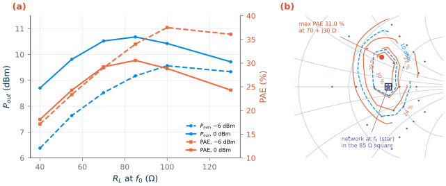
python3 pa_lab.py loadlineThe ideal tuner of Chapter 16 replaces the output network in
\[P_{in} = \frac{\vert V_s\vert^2}{8\cdot 50\ \Omega}, \quad P_{out} = \frac{\vert V_{o,1}\vert^2}{2R_L}, \quad P_{DC} = V_{PA}I_{PA} + V_{B1}I_{B1} + V_{B2}I_{B2}, \quad \mathrm{PAE} = \frac{P_{out} - P_{in}}{P_{DC}},\]out/pa_loadline.cir: a lossless resonator at the collector (8 Ω of reactance at f0) feeds the supply and shorts the harmonics, and a series branch presents \(R_L\) + j0 at f0. The.controlblock runs twelve transients, one for each of six resistances from 40 to 130 Ω at each of two drive levels, −6 and 0 dBm of available input power. Before eachtranit sets the load withalter @rl[resistance] = …and the drive withalter @vs[sin] = [ 0 amp 2.44e9 ]. Each transient lasts 60 periods; ngspice keeps only the last 10 (tran 2.049e-12 2.459e-08 2.049e-08) and writes them as an ASCII raw file.measure()in the script resamples them on 128 points per period and takes the FFT with NumPy [31]: bin 10k of the last 10 periods is harmonic k. From the phasors it computeswith \(P_{in}\) the available power of the 50 Ω source and \(P_{DC}\) including the two base supplies.
-
A small load-pull.
python3 pa_lab.py loadpullThe same tuner, now with a reactance:
out/pa_loadpull.cirsteps the series inductor (alter @lx[inductance]) and the resistor over Chapter 16’s grid of six resistances and five reactances, −60 to +60 Ω, at 0 dBm of drive: 30 transients. The script prints the PAE and output power on the grid and finds their maxima. For the Smith chart it turns each load into a reflection coefficient with scikit-rf [30],rf.tlineFunctions.zl_2_Gamma0(50, Z), interpolates the grid linearly with SciPy [178] and draws the contours in the Γ plane (Figure L7.1b). -
The output network in scikit-rf.
python3 pa_lab.py networkThe published design is in
ch16_numbers.jsonunderpa.offchip_h23.values. The script takes its inductances as published and recomputes the three trap capacitors from their resonance, your Hand calculation 2: the JSON file rounds them to three digits, and C4 = 0.141 pF instead of 0.1414 pF detunes a trap that rejects 66 dB enough to move the second harmonic by 0.3 dB.network()then builds the network of Figure 16.5 as a scikit-rf two-port, port 1 at the collector and port 2 at the 50 Ω load:m = rf.media.DefinedGammaZ0(frequency=freq, z0_port=50) ind = lambda L: rf.Network(frequency=freq, s=rf.network.y2s(C16._ind_y("offchip", L, f), z0=50)) # L + w0L/40 trap = lambda L, C: m.shunt(ind(L) ** m.capacitor(C * 1e-12) ** m.short()) # L-C to ground net = (m.shunt_capacitor(69.7e-15) ** m.shunt(ind(L1) ** m.short()) ** trap(Lt, Ct) ** trap(L3c, C3c) ** ind(L2) ** m.capacitor(Cb * 1e-12) ** trap(L4, C4)) zc = net.s11.z[:, 0, 0] # port 2 matched: the collector's load eff = abs(net.s[:, 1, 0])**2 / (1 - abs(net.s[:, 0, 0])**2) # P_load / P_collectorThe inductors are Chapter 16’s model of an off-chip part, an ideal inductance with a series resistance of ω0L/40, taken from
C16._ind_y()as a Y matrix; the device’s output capacitance, 69.7 fF, is a shunt capacitor at port 1, as in the design. The step prints the collector impedance at f0, 2f0 and 3f0, the network efficiency and the 2f0 and 3f0 rejection (the output voltage per collector current relative to f0, from the Z-parameters), and compares the result with Chapter 16’s own nodal analysis,net_solve(). -
The power sweep.
python3 pa_lab.py sweepout/pa_sweep_offchip_h23.cirputs the network behind the transistors (outnet_lines("offchip", …): each inductor anlin series with anr) and runs 15 transients, −20 to +8 dBm of drive in 2 dB steps. The script prints a row per drive (output power, gain, PAE, collector efficiency, supply current, H2, H3 and the phase of the output relative to the source) and interpolates the operating point at +10 dBm out. P1dB is interpolated where the gain has fallen 1 dB below its value at −20 dBm; AM-PM is the change of the phase from −20 dBm. -
Breakdown. The same step saves the collector, the emitter of Q2 and the base of Q1 for the drive closest to +10 dBm out and for full drive, and prints the peaks of \(v_{CE}\) and \(v_{CB}\) of Q2, \(v_{CE}\) of Q1 and the DC base currents (Figure L7.4).
-
Everything at once.
python3 pa_lab.py allruns steps 1–6, stores the numbers inlab_numbers.jsonand draws Figures L7.1–L7.4 intoout/.
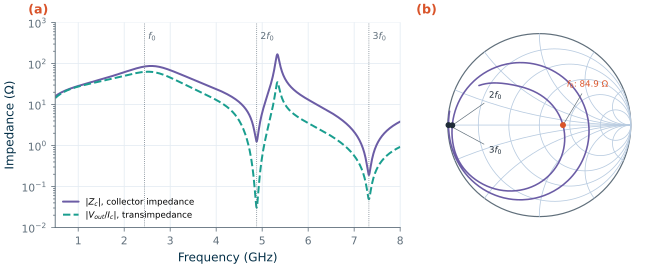
offchip_h23 (Q = 40 inductors, trap capacitors from their resonance) as a scikit-rf two-port with the 69.7 fF of the device at port 1 and 50 Ω at port 2. (a) Collector impedance |Zc| and transimpedance |Vout/Ic|. (b) Zc on the Smith chart; dots at f0, 2f0 and 3f0.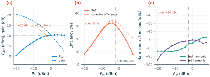
offchip_h23, tt, 27 °C. (a) Pout and gain. (b) PAE and collector efficiency; dashed red: the 30 % specification. (c) Second and third harmonic at the 50 Ω load. Dotted: the drive for +10 dBm out.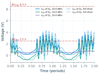
offchip_h23 at 10.0 dBm out (solid) and at +8 dBm of drive (dashed); dash-dotted: the typical BVCEO and BVCBO of npn13G2v.Checkpoint
Table L7.1. Lab 7 results (SG13G2, tt, 27 °C, VPA = 2.0 V; network offchip_h23 unless stated; operating point interpolated at +10 dBm out). Tolerance: ±1 in the last digit shown, except where stated.
| Quantity | Lab 7 | Chapter 16 |
|---|---|---|
| Hand calculation: Ropt for 0.30 dB / 1 dB of network loss (±2 %) | 91 Ω / 78 Ω | 78 Ω (Worked example 16.1) |
| Hand calculation: Ct, C3c, C4; trap reactances at f0 | 0.324, 0.945, 0.141 pF; −150.9, −61.3, −345.9 Ω | 0.324, 0.945, 0.141 pF; −151, −61.3 Ω |
| Hand calculation: the capacitor C4’s trap stands for; loss of a 2f0 / 3f0 trap | 0.189 pF; 0.83 % / 0.31 % | C2 = 0.194 pF (Table 16.2) |
| Hand calculation: PAE from η(1 − 1/G); peak vCE, vCB of Q2 for a sinusoid | 31.7 %; 2.8 V, 2.0 V | |
| Quiescent current; VE2 | 5.67 mA; 0.602 V | 5.67 mA |
| S11, S21 at 2.51 GHz, Chapter 16’s grid point | −12.9 dB, 18.4 dB | −12.9 dB, 18.4 dB (numbers file) |
| Zout, Cdev at 2.51 GHz | 44.3 − j934 Ω, 69.7 fF | 44.3 − j934 Ω, 69.7 fF |
| S11, S21; Zout, Cdev at 2.44 GHz | −13.05 dB, 18.42 dB; 44.9 − j964 Ω, 67.5 fF | −13.0 dB, 18.4 dB |
| μ minimum, 0.1–30 GHz; K minimum, at | 0.99999; −0.49 at 0.1 GHz | 0.99999; −0.49 |
| Load line, −6 dBm: best PAE, at; Pout there | 37.5 % at 100 Ω; 9.56 dBm | 37.5 % at 100 Ω; 9.56 dBm |
| Load line, 0 dBm: best PAE, at; Pout there; Pout at 40 Ω | 30.6 % at 85 Ω; 10.68 dBm; 8.70 dBm | 30.6 % at 85 Ω; 10.68 dBm; 8.70 dBm |
| Load-pull, 0 dBm: maximum PAE and Pout, at | 31.0 %, 10.73 dBm, both at 70 + j30 Ω | 31.0 %, 10.73 dBm, both at 70 + j30 Ω |
| Network: Zc(f0); |Zc| at 2f0, 3f0 | 84.9 + j0.0 Ω; 1.25, 0.19 Ω | 85 Ω (the design’s target) |
| Network efficiency (loss); 2f0, 3f0 rejection | 93.2 % (0.30 dB); −66.2, −62.2 dB | 93.2 % (0.30 dB); −66.3, −62.2 dB (Table 16.2) |
scikit-rf against net_solve(): largest relative difference |
2 × 10⁻¹⁵ | |
| Small-signal gain; P1dB, input and output | 20.35 dB; −15.8, 3.6 dBm | 20.36 dB; −15.8, 3.6 dBm |
| Psat; peak PAE, at Pout | 10.4 dBm; 32.5 % at 9.6 dBm | 10.4 dBm; 32.5 % at 9.6 dBm |
| At +10 dBm: drive; gain | −2.2 dBm; 12.2 dB | −2.2 dBm; 12.2 dB |
| At +10 dBm: PAE; collector efficiency; supply current | 31.0 %; 33.7 %; 14.9 mA | 31.0 %; 33.7 %; 14.9 mA |
| At +10 dBm: H2, H3 | −75.0 dBc, −71.2 dBc | −75.0 dBc, −71.2 dBc |
| AM-PM at +10 dBm; over the whole sweep | −33.6°; −63.4° | −33.6°; −63.4° |
| Breakdown at 10.04 dBm out (−2 dBm drive): peak vC; vCE, vCB of Q2; vCE of Q1 | 4.29 V; 3.58, 2.89 V; 0.757 V | 4.32 V; 3.61, 2.92 V; 0.757 V (3f0 trap only, Table 16.3) |
| Breakdown at full drive (+8 dBm): peak vC; vCE, vCB of Q2; vCE of Q1 | 5.03 V; 4.30, 3.63 V; 0.866 V | 5.05 V; 4.33, 3.65 V; 0.865 V (3f0 trap only) |
| Base currents IB1, IB2: at 10.04 dBm; at full drive (±1 %) | 237, 324 µA; 1116, 1047 µA | 238, 326 µA; 1120, 1050 µA (3f0 trap only) |
Every number that Chapter 16 reports for this PA comes out the same, within ±1 in the last digit, with three remarks. First, the small-signal numbers: Chapter 16 quotes S11 and S21 at 2.44 GHz, but read the output impedance at the point of its 20-per-decade grid nearest to 2.44 GHz, which is 2.51 GHz. The lab gives every one of them at both frequencies. The device capacitance the network absorbs is 69.7 fF in the chapter but 67.5 fF at the carrier itself; that moves the collector’s load by only 0.24 Ω of reactance (Questions). Second, the network: its inductances carry the JSON file’s three digits, so Zc(f0) is 84.9 instead of 85.0 Ω and the 2f0 rejection −66.2 instead of −66.3 dB, and the small-signal gain is 0.01 dB lower; nothing else moves. Third, the breakdown: Chapter 16 published the junction voltages for the collector-trap network only. With the 2f0 trap also at the output, every peak is 0.03 V lower. Run that network yourself in the Extension: our run of it, stored under sweep_offchip_h3 in lab_numbers.json, reproduces Table 16.3 exactly (3.61 and 2.92 V near +10 dBm, H2 −50.7 dBc).
Questions
- Hand calculation 3 gives 31.7 % and the simulation 31.0 %. Find the missing 0.7 points in the printout of step 5: which currents does the PAE charge to the PA that the collector efficiency does not?
- The load line’s PAE optimum moves from 100 Ω at −6 dBm to 85 Ω at 0 dBm of drive, and the load-pull’s from 85 Ω to 70 + j30 Ω. Why does the best load fall as the drive rises, and why is a slightly inductive load better than the purely resistive one?
- The design absorbed 69.7 fF, the capacitance at 2.51 GHz, while the device has 67.5 fF at 2.44 GHz. Put 67.5e-15 as
cdevintonetwork()(import it frompa_lab) and read Zc(f0). Why does a 3 % error in the device capacitance hardly matter for this PA, and for what kind of PA would it? - Rollett’s K is −0.49 at 0.1 GHz, while μ is 0.99999 there, stays within 11 ppm of 1 up to 0.14 GHz and is above 1 from 0.16 GHz on. Print |S22| at 0.1 GHz. What does a reflection coefficient a few parts per million above 1 mean for the output with its ideal 1 µH choke, why does it throw K far below 1 but μ hardly at all, and why would any real bias feed remove it?
- The 2f0 trap at the collector shorts the second harmonic to 1.25 Ω, yet without the output trap the second harmonic is only −50.7 dBc. Why does a second trap at the output, which costs 0.1 points of network efficiency, gain 24 dB?
- Q2’s vCE exceeds BVCEO by 1.1 V at +10 dBm. Section 16.8 names three conditions under which that is acceptable. Which of them does this simulation check, and which can it not?
Extension
Other output networks. --net takes any network of Table 16.2 by its key in ch16_numbers.json. Run python3 pa_lab.py sweep network --net offchip_h3 (the collector trap only) and compare H2, the network’s 2f0 rejection and the peak junction voltages with Table 16.3. Then run python3 pa_lab.py sweep --net chip, the network built from Chapter 7’s spirals: does it reach +10 dBm, and how does its PAE compare with the 23.8 % of Section 16.8? Where in Figure L7.2’s network would you spend a better inductor first?
Another supply. Chapter 16’s first experiment raises VPA to 2.5 V. Run python3 pa_lab.py loadline sweep --vpa 2.5 (the numbers go into lab_numbers.json under loadline_vpa2.5 and sweep_vpa2.5). Where does the load line put the optimum now, compared with Eq. (16.5)? The sweep keeps the network designed for 85 Ω at 2.0 V: how much output power does the higher supply buy, what happens to the PAE at +10 dBm, and how close do Q2’s vCE and vCB now come to their limits? What would you change in the network first?