Chapter 11
LC Oscillators and Phase Noise
Every channel the course radio sends or receives is defined by one oscillator. This chapter builds it: an LC tank whose losses a cross-coupled pair cancels, a capacitor bank and a varactor that tune it across the band in every corner, and the theory that predicts its phase noise, from Leeson's model to the impulse sensitivity function. We measure that function for every noise source of the course VCO with ngspice transients, take each transistor's noise at every instant of the cycle from frozen noise analyses, and add them up. The result is a 4.8 GHz VCO for the synthesizer of Part IV that covers its band in the slow and fast corners and meets its phase-noise budget with 12.7 dB to spare, at 0.766 mW. A counter-based calibration then picks its bank code for every channel, and a last section simulates the oscillators the course does not build: a quadrature VCO, and the push-push, coupled and standing-wave alternatives.
- Explain oscillation as a feedback loop and as a negative resistance, and check the start-up margin of a cross-coupled LC oscillator.
- Calculate the Q of an LC tank from its inductor, varactor and switched capacitors, and identify the element that limits it.
- Size a cross-coupled VCO with a capacitor bank and a varactor that covers a band over process and temperature with a chosen KVCO, and calibrate its band automatically.
- Predict phase noise with Leeson’s model and with the impulse sensitivity function, and simulate it for every noise source of an oscillator from measured ISFs and frozen noise analyses.
- Compare oscillators with a figure of merit, specify a VCO for a PLL, and weigh quadrature, push-push, coupled and standing-wave oscillators against it.
Contents
- 11.1 Oscillation: feedback and negative resistance
- 11.2 The LC tank and its Q
- 11.3 The cross-coupled LC VCO
- 11.4 Colpitts and HBT oscillators
- 11.5 Tuning: varactors, capacitor banks and KVCO
- 11.6 Phase noise: Leeson’s model
- 11.7 Phase noise: the impulse sensitivity function
- 11.8 The course VCO at 4.8 GHz
- 11.9 Other oscillators
- Further reading
11.1 Oscillation: feedback and negative resistance
The PLL chapter of The Art of Analog IC Design built a ring oscillator: a loop of inverters whose delay sets the frequency. A ring is small and tunes over a decade, but every edge is the charging of a capacitor by a noisy transistor current, and nothing filters that noise. An LC oscillator replaces the delay by a resonator. The tank stores energy and returns it once per cycle, so the noise only has to perturb a small fraction of that energy. That is why every radio synthesizer, including the course’s, uses one.
Two views of the same circuit
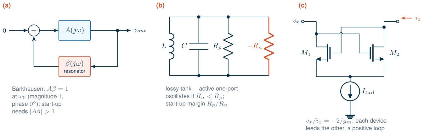
The first view is a feedback loop (Figure 11.1a): an amplifier \(A\) and a frequency-selective network \(\beta\) in a loop with no input. A signal that goes once round the loop and returns with the same amplitude and phase sustains itself. This is the Barkhausen criterion:
\[A(j\omega_0)\,\beta(j\omega_0) = 1. \tag{11.1}\]The resonator makes the phase condition hold at one frequency only, \(\omega_0\). At start-up the loop gain must be larger than one, so that noise (or, in a simulator, a kick) grows; the amplifier’s nonlinearity then reduces the average gain until Eq. (11.1) holds and the amplitude settles [6, 7].
The second view suits LC oscillators better (Figure 11.1b). A real tank is an inductor \(L\) and a capacitance \(C\) whose losses can be lumped into a parallel resistance \(R_p\):
\[\omega_0 = \frac{1}{\sqrt{LC}}, \qquad Q = \frac{R_p}{\omega_0 L} = \omega_0 R_p C, \qquad R_p = Q\,\omega_0 L. \tag{11.2}\]Left alone, a tank rings down: each cycle \(R_p\) dissipates \(2\pi/Q\) of the stored energy (Chapter 7, Eq. 7.1). A one-port with a negative resistance \(-R_n\) in parallel delivers power instead. If \(R_n < R_p\), the net parallel resistance is negative and the oscillation grows; it stops growing when the active circuit’s large-signal resistance, averaged over a cycle, has risen to exactly \(-R_p\). The ratio \(R_p/R_n\) of the small-signal values is the start-up margin. Designers keep it at two to three in the worst corner, because it falls with temperature and slow transistors, and because a large margin pushes the circuit deeper into the nonlinear regime, which costs noise.
The cross-coupled pair
The negative resistance of almost every integrated LC oscillator is a cross-coupled pair (Figure 11.1c). Drive a small current \(i_x\) into the drains: \(M_1\)’s gate sees \(+v_x/2\) and \(M_2\)’s gate \(-v_x/2\), so \(M_1\) draws \(g_m v_x/2\) more and \(M_2\) \(g_m v_x/2\) less, a current that flows out of the node into which \(i_x\) flows in. The pair answers a voltage with a current of the wrong sign:
\[R_{in} = -\frac{2}{g_m}, \qquad \text{start-up: } \frac{g_m}{2} \ge \frac{1}{R_p}. \tag{11.3}\]Each transistor is a common-source amplifier whose load is the tank and whose input is the other transistor’s output: a two-stage loop with two inversions, the feedback view of the same circuit. A complementary pair adds a PMOS cross-coupled pair in parallel, and its conductance becomes \(-(g_{mn} + g_{mp})/2\).
Worked example 11.1 · Start-up margin of the course VCO
The course tank of Section 11.2 has \(R_p\) = 906 Ω at 4.868 GHz, so the pair must provide at least \(1/R_p\) = 1.1 mS. An ngspice operating point and ac analysis of the course pairs at 4.88 GHz, with an ideal tail current of 0.6 mA, gives 1.38 mS for the NMOS pair alone (16 µm/0.13 µm devices) and 2.88 mS with the PMOS pair added (Figure 11.5a): start-up margins of 1.2 and 2.6. The complementary pair starts at 0.152 mA; the NMOS pair alone needs 0.441 mA.
11.2 The LC tank and its Q
The tank sets the oscillator’s frequency, and its Q sets how much of every noise source becomes phase noise (Section 11.6): phase noise falls as \(1/Q^2\). The losses of the tank’s elements add as conductances. With the capacitance split into elements \(C_i\) of quality factor \(Q_i\) out of a total \(C\),
\[\frac{1}{Q_{tank}} = \frac{1}{Q_L} + \sum_i \frac{C_i}{C}\,\frac{1}{Q_i}, \tag{11.4}\]so a lossy capacitor matters only in proportion to its share of the tank capacitance. Chapter 7 characterized each candidate element at 4.88 GHz: the EM-fitted L3 spiral (1.98 nH, differential Q 17.7), the sg13_hv_svaricap varactor (Q ≥ 89 at \(L\) = 0.3 µm), MIM capacitors (Q in the hundreds for a small plate with a wide feed) and switched capacitors, whose Q is traded against tuning range through the switch width (Eq. 7.11).
Figure 11.2 applies Eq. (11.4) to the tank of the course VCO (Section 11.8), simulated element by element in ngspice at the oscillation frequency, each biased as in the oscillator. The inductor has Q = 17.8 and causes 84 % of the loss. The capacitor bank, a quarter of the tank capacitance at the middle code with Q = 21.6, adds 10 %. The varactor (Q = 98.3), the fixed MIM capacitors (Q = 394) and the divider input (Q = 12.2, but only 7.61 fF) share the rest. The tank Q is 14.9, \(R_p\) = 906 Ω and the differential capacitance 537 fF.
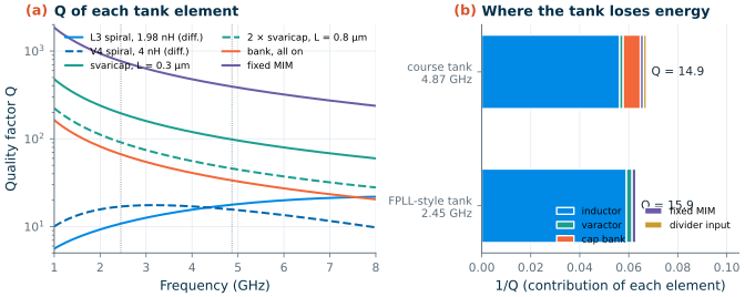
The same analysis of a tank like that of the taped-out SG13G2 2.4 GHz PLL of Thiriloganathan et al. [106, 207] (the V4 model of its 4 nH spiral from Chapter 7, two svaricaps with \(L\) = 0.8 µm and \(N_x\) = 7, and a 21.9 µm cap_rfcmim with a 10 µm feed) gives Q = 15.9 at 2.45 GHz, of which 94 % of the loss is in the inductor (Q = 16.9). Their 0.8 µm varactors have Q = 91.1 at 2.45 GHz, high enough because Q scales as \(1/\omega\) for a series resistance. In both tanks, a factor of two apart in frequency, the tank Q is the spiral’s Q within about 15 %.
What this means for your design
In SG13G2 at 2.4–5 GHz a tank Q of 15 to 16 is what a well-designed spiral gives, and the varactor and MIM capacitors cost little. The element to watch is the switched-capacitor bank: its switches must be wide enough not to spoil the Q (Eq. 7.11), and its off-state capacitance, which does not tune, grows with the width. A tank Q is only as good as its EM model: Chapter 7 found its inductances within a few per cent of an independent HFSS result, and Section 11.5 leaves tuning range for that uncertainty.
11.3 The cross-coupled LC VCO
NMOS-only or complementary
Two topologies dominate. The NMOS-only oscillator connects the inductor’s centre tap to \(V_{DD}\) and an NMOS cross-coupled pair to the two ends, with a tail current source below. Each output swings around \(V_{DD}\), up to about \(V_{DD}\) above it. The complementary oscillator puts a PMOS pair on top and an NMOS pair below the same tank, and needs no centre tap (Figure 11.3). In both, the tail current \(I\) is switched from side to side; when the pair switches completely, the current through the tank is a square wave whose fundamental sets the amplitude. In the complementary circuit the full current reverses direction through the tank every half period, which doubles the fundamental [122]:
\[V_A \approx \frac{4}{\pi}\,I R_p \ \text{(complementary)}, \qquad V_A \approx \frac{2}{\pi}\,I R_p \ \text{(NMOS-only)}, \tag{11.5}\]where \(V_A\) is the peak of the differential voltage. These amplitudes hold in the current-limited regime. When \(V_A\) approaches what the supply allows, the transistors enter the triode region at the peaks, the tail loses its headroom, and the amplitude saturates: the voltage-limited regime, in which more current only adds noise [122, 126]. For the same current, the complementary circuit gives twice the swing, which is why it is the usual choice at a 1.2 V supply. Its PMOS devices add capacitance (the pair loads the tank with 99.5 fF against 35.7 fF for the NMOS pair alone, Section 11.4), and its swing is limited to about \(V_{DD}\) differential, against about \(2V_{DD}\) for the NMOS-only circuit.
tools/figs/_ch11_vco.py.The course VCO
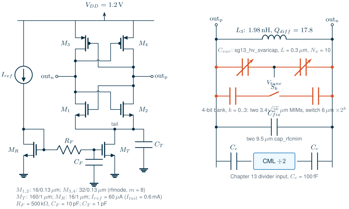
Figure 11.3 shows the circuit that Section 11.8 completes. The tank is Chapter 7’s L3 spiral with the varactor, the bank, two fixed 9.5 µm MIM capacitors that bring the frequency down to the band, and the Chapter 13 divider’s clock inputs. \(M_1\)–\(M_4\) are minimum-length devices with the RF model switched on (rfmode=1) and split into \(m\) = 8 instances, which divides the model’s fixed 40 Ω gate resistance by eight (Chapter 6); the PMOS devices are twice as wide as the NMOS devices, to give the two pairs similar transconductance. A 1:10 mirror sets the tail current, and a 500 kΩ–10 pF filter (a 32 kHz pole) keeps the reference’s noise away from the tail gate. The 1 pF tail capacitor shorts the tail node at \(2\omega_0\), where the pair’s common node swings.
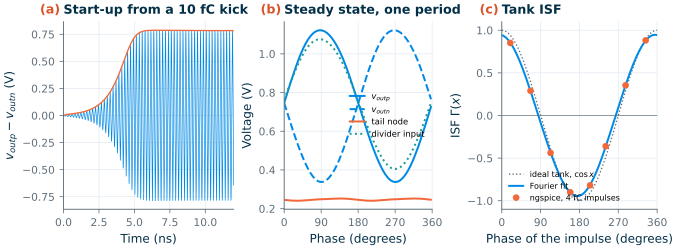
Figure 11.4 shows the transient. A 10 fC kick starts the oscillation, the envelope grows exponentially, and after 5 ns the amplitude is within 10 % of its final value. At bank code 8 and \(V_{tune}\) = 0.6 V the oscillator runs at 4.868 GHz with a differential amplitude of 0.784 V (0.392 V on each side, around a common-mode level of 0.739 V) and draws 0.639 mA, 0.766 mW from 1.2 V, reference branch included. After its 100 fF coupling capacitor the divider sees 0.335 V, 3.4 times the 100 mV it needs at 4.8 GHz (Chapter 13).
Eq. (11.5) predicts \(V_A\) = 0.692 V for the nominal 0.6 mA, close to the simulated 0.784 V: the circuit runs in the current-limited regime, where the amplitude, and with it the phase noise of Section 11.6, scales with the current. Doubling the current would bring it near the 1.2 V supply’s limit, where it saturates.
11.4 Colpitts and HBT oscillators
The cross-coupled pair is not the only way to make a negative resistance. The Colpitts oscillator uses one transistor and a capacitive divider \(C_1\), \(C_2\) across the tank: the source (or emitter) follows the gate, and the divider feeds back enough of the output to make the input resistance negative [6]:
\[R_{in} = -\frac{g_m}{\omega^2 C_1 C_2}. \tag{11.6}\]Referred to the tank, the divider transforms this by its ratio, and the Colpitts needs several times the transconductance of a cross-coupled pair to start. In return its transistor conducts only in a short pulse near the bottom of each cycle, when the ISF of Section 11.7 is small, so it converts its own noise inefficiently into phase noise. Andreani et al. [127] showed that, at equal power and tank Q, the CMOS Colpitts still does not beat the cross-coupled oscillator, whose noise is shared by more efficient switching; the Colpitts survives where a single-ended oscillator or a resonator on one terminal is wanted, as in crystal oscillators.
The SiGe HBT changes the comparison in two ways (Figure 11.5). First, its transconductance per current is the highest of any device, \(g_m = I_C/V_T\): at 0.6 mA an npn13G2 cross-coupled pair gives 5.06 mS of negative conductance at 4.88 GHz, 3.7 times the NMOS pair’s 1.38 mS, and loads the tank with 26.1 fF instead of 35.7 fF. Second, and more important for phase noise, its flicker noise is tiny. An NMOS of the course pair at 0.3 mA has a drain-noise flicker corner of 11500 kHz; an npn13G2 at the same current has 0.232 kHz (both driven from the 1.75 Ω DC resistance of the spiral). Section 11.7 shows that the 1/f³ corner of the phase noise is proportional to the device’s flicker corner (Eq. 11.12), so HBT oscillators are the choice when close-in phase noise matters. (In the course VCO, Section 11.7 finds that the transistors’ flicker noise alone would put that corner at 65 kHz.)
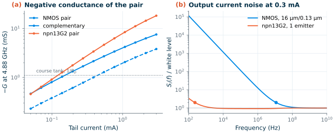
The catch is headroom. The npn13G2 needs \(V_{BE}\) ≈ 0.825 V at 0.3 mA. In a cross-coupled HBT pair the base of each device sits at the other’s collector, so at a 1.2 V supply the collector–base junction is at zero bias at rest and forward-biased on every negative peak: the swing is limited to a few hundred millivolts before the devices saturate. Practical HBT VCOs couple the bases capacitively and bias them separately, use a higher supply (SG13G2’s HBTs tolerate it), or use the Colpitts form, which is why they dominate at millimetre waves (Chapter 17) and in high-performance synthesizers. For the course radio, with a 1.2 V supply and a PLL that suppresses the VCO’s close-in noise (Chapter 12), the CMOS circuit is the economical choice.
11.5 Tuning: varactors, capacitor banks and KVCO
A VCO tunes by changing the tank capacitance. With \(C_{var}(V_{tune})\) part of the total \(C\), Eq. (11.2) gives the tuning gain
\[K_{VCO} = \frac{\partial f}{\partial V_{tune}} = -\frac{f_0}{2C}\,\frac{\partial C_{var}}{\partial V_{tune}}. \tag{11.7}\]\(K_{VCO}\) sets the PLL’s loop gain (Chapter 12), and it converts every microvolt of noise on the tuning line into frequency noise. A varactor that alone covered the band with process margin would need a large \(K_{VCO}\). The course VCO therefore splits the job: a switched-capacitor bank chooses one of 16 bands, and a small varactor tunes within each band.
How wide must the coverage be? The band is 4.802–4.962 GHz (Chapter 5), 3.3 % wide. Around it come the uncertainties: the spiral’s inductance (Chapter 7 found 8 % between two EM solvers, ±4 % in frequency), the MIM capacitance and the transistor capacitances over process, and temperature. We aim for about ±7 %, roughly 4.55–5.25 GHz, with bands that overlap, so that every channel lies well inside some band.
Worked example 11.2 · Sizing the varactor and the bank
With \(C\) ≈ 537 fF, the band edges (4.55 and 5.25 GHz) need a capacitance range of \((5.25/4.55)^2\) = 1.33. The varactor, one
sg13_hv_svaricapwith \(L\) = 0.3 µm and \(N_x\) = 10 between the outputs, has a small-signal capacitance from 87.3 fF to 59.2 fF as \(V_{tune}\) goes from 0 to 1.2 V (its gates sit at the oscillation’s mean 0.739 V); its steepest slope, 39.7 fF/V, predicts by Eq. (11.7) a peak \(K_{VCO}\) of 180 MHz/V. The bank’s LSB is two 3.4 µm MIM plates in series with a 6 µm switch, and each bit doubles both; the bank’s differential capacitance rises from 23.4 fF at code 0 to 132 fF at code 15 (where its Q is 33.6).
With these element values, Eq. (11.2) gives a first estimate of the coverage: referred to the transient at code 8 and 0.6 V, the frequency scales as \(\sqrt{C/(C + \Delta C)}\), with \(\Delta C\) the change of the bank’s and the varactor’s simulated capacitance. The 16 bands then span 4.622–5.264 GHz at the typical corner, about 32.6 MHz per code, while the varactor tunes each band by 113 MHz (code 15) to 154 MHz (code 0). The mean \(K_{VCO}\) over 0–1.2 V is about 94.3 MHz/V at code 15, 108 MHz/V at code 8 and 129 MHz/V at code 0, larger at the top of the range, where the varactor is a larger part of a smaller tank (Eq. 11.7).
Common pitfall · Trusting a small-signal tuning curve
The estimate uses the varactor’s small-signal C–V. The oscillator sees something else: its outputs swing by ±0.392 V, so the varactor sweeps through much of its C–V curve every cycle and the tank sees an average capacitance. The large-signal tuning curve is flatter, and its \(K_{VCO}\) smaller near the steepest point. Before handing \(K_{VCO}\) and the coverage to the PLL designer, measure them with transients (or PSS) at the real amplitude, for every code and in every corner.
The tuning range, simulated
We did that (Figure 11.6). Each of 96 ngspice transients starts the VCO with a kick and measures its frequency over the last 8 ns of 20 ns: every bank code at \(V_{tune}\) = 0, 0.6 and 1.2 V and codes 0, 8 and 15 every 0.1 V at the typical corner, and codes 0, 8 and 15 at 0, 0.6 and 1.2 V in a slow corner (ss transistors, cap_wcs capacitors, 85 °C) and a fast corner (ff, cap_bcs, −40 °C). The spiral keeps its EM model in all of them.
At the typical corner the 16 bands span 4.633–5.224 GHz: the bottom 0.25 % above the estimate, the top 0.8 % below it. The bands are 30.4 MHz apart on average and 103 MHz (code 15) to 136 MHz (code 0) wide, so each overlaps its neighbour by at least 72 % of a band. The slow corner shifts the range down to 4.516–5.110 GHz, the fast corner up to 4.753–5.340 GHz. The course band, 4.802–4.962 GHz, is covered in all three, with 3.5 % to spare below it and 5.3 % above at the typical corner, but only 1.0 % below in the fast corner and 3.0 % above in the slow corner. Those margins are smaller than the ±4 % in frequency that Chapter 7’s inductance uncertainty allows: a spiral 8 % below its model in a fast lot would lose the lowest channels. Adding about 10 fF of fixed capacitance (2 % of the tank’s) would centre the range, with 2.0 % to spare at each end in the corners; covering the inductance uncertainty as well needs a wider bank, whose larger switches cost Q (Eq. 7.11). The oscillator starts in both corners, with amplitudes from 0.668 V (slow, code 15) to 0.871 V (fast, code 0), and draws 0.614–0.652 mA.
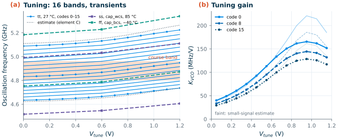
The tuning gain is lower and less constant than the estimate, as the pitfall above warned. The mean \(K_{VCO}\) over 0–1.2 V is 113, 96.9 and 85.6 MHz/V at codes 0, 8 and 15, 9–12 % below the small-signal values; at code 8 it is 84.6 MHz/V in the slow corner and 112 MHz/V in the fast one. Across the tuning range it varies by a factor of four: at code 8 from 34 MHz/V near 0 V to 144 MHz/V near 0.95 V. Section 11.8 calibrates the band so that \(V_{tune}\) settles on the steep part of the curve; over every channel and corner the loop then sees 103–167 MHz/V, still a 1.6:1 spread in loop gain, which Chapter 12 must tolerate.
For two-point modulation (Chapter 5), the GFSK deviation of ±250 kHz at the LO is ±500 kHz at the VCO, a few millivolts on the tuning line at this \(K_{VCO}\): small enough to stay on the locally linear part of the curve.
11.6 Phase noise: Leeson’s model
An ideal oscillator’s spectrum is a line. Noise perturbs the zero crossings of a real one, which spreads its power into skirts around the carrier. The phase noise \(\mathcal{L}(\Delta f)\) is the power in 1 Hz at an offset \(\Delta f\), relative to the carrier, in dBc/Hz; for small deviations it is half the spectral density of the phase, \(S_\phi(\Delta f)/2\). The sibling course related it to jitter (The Art of Analog IC Design, Section 23.3), and Chapter 5 derived the course’s requirement from reciprocal mixing: −110 dBc/Hz at 1 MHz at the LO, −104.0 dBc/Hz at the VCO.
Leeson’s model [120] explains the shape of the spectrum with a linear argument. Noise of density \(2FkT\) (a noise factor \(F\) times the thermal noise) at the input of a resonator of loaded \(Q\) in a loop is integrated by it within its half-bandwidth \(f_0/2Q\), so the phase wanders:
\[\mathcal{L}(\Delta f) = 10\log_{10}\!\left[\frac{2FkT}{P_{sig}}\left(1 + \left(\frac{f_0}{2Q\,\Delta f}\right)^2\right)\left(1 + \frac{\Delta f_{1/f^3}}{\Delta f}\right)\right]. \tag{11.8}\]The first factor is noise relative to signal; the second a \(1/\Delta f^2\) (−20 dB/decade) region inside the resonator’s bandwidth; the third an empirical \(1/\Delta f^3\) (−30 dB/decade) region below a corner \(\Delta f_{1/f^3}\). For a differential tank, with \(P_{sig} = V_A^2/2R_p\) and in the \(1/f^2\) region,
\[\mathcal{L}(\Delta f) = 10\log_{10}\!\left[\frac{F\,kT R_p}{V_A^2}\left(\frac{f_0}{Q\,\Delta f}\right)^2\right]. \tag{11.9}\]Worked example 11.3 · Leeson’s estimate for the course VCO
With \(R_p\) = 906 Ω, \(Q\) = 14.9, \(V_A\) = 0.784 V and \(f_0\) = 4.868 GHz, Eq. (11.9) gives −121.8 dBc/Hz at 1 MHz for \(F\) = 1, the noise of the tank alone. The specification of −104.0 dBc/Hz allows an \(F\) of up to 69. But what is \(F\)? Leeson’s model does not say: it is a fitting factor that lumps the transistors’ noise, the way the circuit samples it, and the conversion of flicker noise, which Eq. (11.8) only describes with an empirical corner. Section 11.7 simulates it: for this VCO, \(F\) = 3.71 at 1 MHz.
The model still teaches the design rules. In the current-limited regime \(V_A \propto I\), so the phase noise falls 6 dB for every doubling of the current, while the power doubles: the figure of merit (Section 11.8) stays the same. In the voltage-limited regime \(V_A\) stops growing and the extra current only adds noise. And for a given inductor technology, \(R_p/Q^2 = \omega_0 L/Q\): a larger inductance gives a larger swing for the current, but more noise per volt of swing.
11.7 Phase noise: the impulse sensitivity function
The idea
Hajimiri and Lee [121] replaced the fitting factor by a measurement. Inject a small charge \(\Delta q\) into a node of an oscillator at some instant. The disturbance changes both the amplitude and the phase. The oscillator’s limiting restores the amplitude within a few cycles, but nothing restores the phase: the oscillator carries on, shifted for ever. The shift is proportional to the charge and depends on when in the cycle it arrives:
\[\Delta\phi = \Gamma(\omega_0\tau)\,\frac{\Delta q}{q_{max}} = h(\omega_0\tau)\,\Delta q, \tag{11.10}\]where \(\Gamma(x)\) is the impulse sensitivity function (ISF), a periodic function of the phase \(x\), normalized to the maximum charge swing \(q_{max} = C V_A\), and \(h = \Gamma/q_{max}\) the same in radians per coulomb. For an ideal LC tank, charge injected at a peak of the voltage changes only the amplitude (\(\Gamma\) = 0), while charge injected at a zero crossing shifts the phase most (\(\lvert\Gamma\rvert\) = 1): with \(x\) measured from a rising zero crossing, \(\Gamma(x) = \cos x\).
A white noise current is a stream of such impulses. Integrated over many cycles, only the rms value of \(\Gamma\) matters for the \(1/f^2\) region, and its DC value for the up-conversion of low-frequency noise. For a source of one-sided density \(\overline{i_n^2}/\Delta f\),
\[\mathcal{L}(\Delta f) = 10\log_{10}\!\left[\frac{\Gamma_{rms}^2}{q_{max}^2}\,\frac{\overline{i_n^2}/\Delta f}{2\,\Delta\omega^2}\right], \tag{11.11}\]and the noise of a transistor that switches on and off is cyclostationary: its density follows the device’s operating point around the cycle, \(\overline{i_n^2}(x) = \overline{i_{n0}^2}\,\alpha^2(x)\), with a noise modulating function \(\alpha(x)\). It enters through an effective ISF, and the flicker noise, which is slow, through the DC part of it [121, 122]:
\[\Gamma_{eff}(x) = \Gamma(x)\,\alpha(x), \qquad \Delta f_{1/f^3} = \Delta f_{1/f}\left(\frac{\Gamma_{eff,dc}}{\Gamma_{eff,rms}}\right)^2. \tag{11.12}\]A symmetric waveform makes \(\Gamma_{eff,dc}\) small, which is why a complementary oscillator with balanced rise and fall has a low 1/f³ corner, and why the HBT’s flicker corner of Section 11.4 is worth so much.
Measuring the ISF in ngspice
Neither ngspice nor Xyce computes phase noise directly (Chapter 2). The ISF, however, is a transient experiment. One transient of the course VCO receives eight charge impulses of 4 fC across the tank, each 2 ps long, spaced by 20 periods and each 1/8 of a period later in phase than the one before. Before and after each impulse, a straight-line fit to 2 ns of zero crossings gives the period and the time shift; the phase step is \(-2\pi\) times the shift over the period. The fits leave at most 2.6 fs rms (the first impulse, still close to start-up), against shifts of up to 270 fs, and the amplitude has settled within 2 ns. The largest step is 8.56 mrad, about 1 % of the charge swing: small enough to be linear.
Figure 11.4c shows the result. The tank’s ISF is the sinusoid that theory predicts, with its peaks at the zero crossings of the differential output. Normalized with \(q_{max} = C V_A\) = 421 fC, it peaks at \(\Gamma\) = 0.946 and has an rms value of 0.664 (an ideal cosine: 1 and 0.707) and a DC value of 0.0034. The peak is slightly below one because part of the injected charge goes into the transistors’ and the bank’s capacitances rather than the tank’s.
The tank’s noise
With the measured ISF, Eq. (11.11) turns the tank’s own noise, \(4kT/R_p\), into −122.4 dBc/Hz at 1 MHz, within a decibel of Leeson’s \(F\) = 1 estimate: for a sinusoidal ISF the two are the same calculation. The transistors add their own noise. A common shortcut brackets their share with a noise factor of a few [122, 124], say \(F\) = 2–5, which would give −119.4 to −115.4 dBc/Hz at 1 MHz; an earlier version of this chapter stopped there. The rest of this section replaces that assumption by a simulation of every noise source.
Every noise source has its own ISF
Every noise current in the oscillator flows between two of four nodes: \(out_p\), \(out_n\), the tail node, and ground or \(V_{DD}\), which the ideal supply holds still. The phase response is linear in small charges, so a charge that leaves node \(a\) and enters node \(b\) shifts the phase by \([h_b(x) - h_a(x)]\,\Delta q\), where \(h_a\) is the ISF of a charge injected into node \(a\) from ground. Three node ISFs therefore describe every source:
| Source | Between | ISF \(h(x)\) |
|---|---|---|
| tank losses, \(4kT/R_p\) | \(out_p\) and \(out_n\) | \(h_{out_p} - h_{out_n}\) |
| NMOS \(M_1\) (\(M_2\)) | \(out_n\) (\(out_p\)) and tail | \(h_{out_n} - h_{tail}\) (\(h_{out_p} - h_{tail}\)) |
| PMOS \(M_3\) (\(M_4\)) | \(V_{DD}\) and \(out_n\) (\(out_p\)) | \(h_{out_n}\) (\(h_{out_p}\)) |
| tail \(M_T\) and its bias network | tail and ground | \(h_{tail}\) |
Five more transients measure them: 24 impulses each, 30 periods apart, of +8 fC and −8 fC into \(out_p\), +8 fC into \(out_n\), and ±20 fC into the tail node, with the same fits as before (over 2.5 ns before each impulse and from 3 ns after it). The fits leave at most 4.3 fs rms, and the largest steps are 9.2 mrad at the outputs and 4.3 mrad at the tail. The responses to +8 fC and −8 fC differ by 1.7 % rms, a second-order effect that their mean cancels, and the mean ISF of \(out_n\) is that of \(out_p\) half a period later within 0.9 %, as the circuit’s symmetry requires. Figure 11.7a shows the result. Each output node has \(\Gamma_{rms}\) = 0.333, and their difference, the tank’s ISF, has 0.666, against 0.664 from the direct measurement of Figure 11.4c. The tail’s ISF is almost constant: \(\Gamma_{dc}\) = 0.0588 against \(\Gamma_{rms}\) = 0.0626, with a ripple at twice the oscillation frequency. A charge into the tail changes the pair’s current and so the amplitude, and the varactor and the transistors’ voltage-dependent capacitances turn the amplitude change into a frequency change: AM-to-PM conversion, whatever the phase of the impulse.
Cyclostationary noise from frozen operating points
A transistor in the oscillator does not have one noise density: its noise follows its operating point around the cycle. An ngspice transient cannot show it, because its transistors are noiseless (Chapter 2), and neither ngspice nor Xyce has a periodic noise analysis for an oscillator. But the oscillation is slow compared with the core transistors’ own time constants, so at each instant a device sits in a quasi-static operating point. We take 128 instants of one period of the steady state (Figure 11.4b) and at each run an ngspice operating point and noise analysis of each core device alone, its terminals held by DC sources at that instant’s voltages: the PSP model’s channel thermal and flicker noise, plus the noise of the gate resistance that rfmode=1 adds. The short-circuit drain current noise is the source to inject between the device’s drain and source.
Figure 11.7b shows the white part. \(M_1\) conducts only while \(v_{outp} > v_{outn}\). Its current averages 0.290 mA, half the tail current, but peaks at 0.923 mA, because the tail capacitor supplies current at twice the oscillation frequency; at the peak of the swing \(M_1\) is in deep triode. Its white drain noise peaks at 157 pA²/Hz. The PMOS devices, twice as wide, peak at 285 pA²/Hz, 1.8 times as much. Both devices also have strong flicker noise: averaged over the cycle, their flicker corners are 7.3 MHz (NMOS) and 16.3 MHz (PMOS). The tail device’s drain moves by only 11 mV, so its noise is stationary; but at 2\(f_0\) its density is 2.8 times its white level at 100 MHz (the PSP model’s drain noise of this long, 1 µm device rises above about 1 GHz), and the bias network adds the thermal noise of the 500 kΩ filter resistor through the 32 kHz pole.
The ISF of each source times its modulating function is its effective ISF (Figure 11.7c). For \(M_1\), \(\Gamma_{eff,rms}\) = 0.141 and \(\Gamma_{eff,dc}\) = −0.011: the device makes its noise while the ISF goes through a zero and a peak of both signs, and the waveform’s symmetry nearly cancels the DC part.
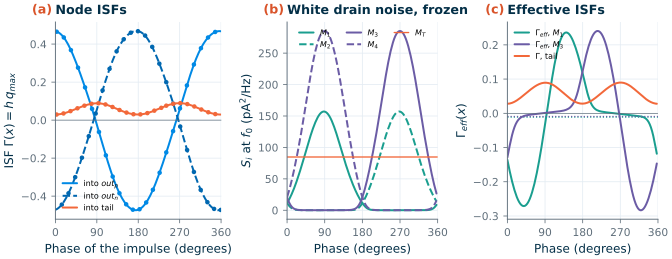
.noise of the device alone at 128 instants; M2, M4 by symmetry). (c) Effective ISFs Γ(x)α(x) of M1 and M3 (α normalized to 1 at its peak; dotted: their DC values) and the tail ISF. Code 8, Vtune = 0.6 V, tt, 27 °C.For each source \(k\) with ISF \(h_k(x)\) in rad/C, white density \(S_{w,k}(x)\) and flicker density \(S_{f,k}(x,\Delta f)\), Eqs. (11.11) and (11.12) become one sum. The white noise is uncorrelated from instant to instant, so its density adds with the weight \(h_k^2\); the flicker noise is slow, so it acts as a slowly varying current shaped by the operating point, and only its average effect over a cycle survives [121]:
Key equation · Phase noise of an oscillator from all its noise sources
\[\mathcal{L}(\Delta f) = \frac{1}{2\Delta\omega^2}\sum_k\left[\Big\langle h_k^2(x)\,S_{w,k}(x)\Big\rangle + \Big\langle h_k(x)\sqrt{S_{f,k}(x,\Delta f)}\Big\rangle^2\right] \tag{11.13}\]where \(\langle\cdot\rangle\) is the average over one period. The first term is Eq. (11.11) with \(\Gamma_{eff,rms}\), the second the up-conversion through \(\Gamma_{eff,dc}\) of Eq. (11.12). A stationary source whose density changes with frequency (here the tail) uses its density at each harmonic of \(f_0\) where its ISF has a component.
The DC part, the flicker term, is a small difference of large numbers, so we also measure it directly. A slow current shaped by the flicker modulating function \(\alpha_f(x)\) is, for the oscillator, a constant current \(I_0\,\alpha_f(x)\), which shifts the frequency by \(\langle h\,\alpha_f\rangle I_0/2\pi\). A behavioural source in ngspice reproduces \(\alpha_f(x)\) exactly as two tables of \(v_{outp} - v_{outn}\), one for each half of the cycle, chosen by the sign of its time derivative; with \(I_0\) = ±20 µA at each site, the frequency moves by ±97 kHz at \(M_1\), ±80 kHz at \(M_3\) and ±0.51 MHz for a current into the tail. These DC values differ from the impulse ISFs’ by +4 % (\(M_1\)), −10 % (\(M_3\)) and +14 % (tail), and we use them in the flicker term. Part of the difference is a response that settles more slowly than the impulse fits assume: fitting the tail’s impulses from 8 ns instead of 3 ns after each raises its \(\Gamma_{dc}\) from 0.060 to 0.063, towards the 0.067 of the DC injection. The tail’s value is the oscillator’s frequency pushing by its tail current: 25.4 MHz/mA.
The simulated phase noise
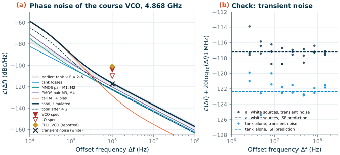
Figure 11.8a adds up Eq. (11.13). At 1 MHz the course VCO has −116.7 dBc/Hz. The tank causes 27 % of it, the NMOS pair 22 %, the PMOS pair 44 % and the tail 7 %. The result lies inside the old bracket of \(F\) = 2–5, 1.3 dB below its pessimistic end: the noise factor that Leeson’s Eq. (11.9) needs to reproduce it is F = 3.71 (3.30 for the white noise alone). The VCO meets its −104.0 dBc/Hz with 12.7 dB to spare, and after the divide-by-two the LO at 2.44 GHz has −122.7 dBc/Hz at 1 MHz, against its −110 dBc/Hz specification.
Table 11.1. Phase noise of the course VCO by source at 1 MHz, each group's share at 1 MHz and 100 kHz, and the 1/f³ corner each group would give on its own (Eq. 11.13; code 8, Vtune = 0.6 V, 4.868 GHz, tt, 27 °C).
| Source | White, dBc/Hz | Flicker and bias, dBc/Hz | Total, dBc/Hz | Share at 1 MHz | Share at 100 kHz | Own 1/f³ corner |
|---|---|---|---|---|---|---|
| Tank losses | −122.4 | — | −122.4 | 27 % | 5 % | — |
| NMOS pair M1, M2 | −123.5 | −135.4 | −123.2 | 22 % | 6 % | 64 kHz |
| PMOS pair M3, M4 | −120.7 | −131.3 | −120.3 | 44 % | 14 % | 87 kHz |
| Tail MT and bias network | −135.4 | −129.5 | −128.5 | 7 % | 75 % | 2.1 MHz |
| Total | −117.2 | −126.7 | −116.7 | 100 % | 100 % | 254 kHz |
The PMOS pair is the largest single contributor. It conducts as the NMOS pair does, in the other half of the cycle and through nearly the same ISF, but the PSP model gives its wider devices 1.8 times the white noise density. In the white region the two pairs together add 2.3 times the tank’s own noise.
Below a 1/f³ corner of 254 kHz the phase noise rises faster than 20 dB per decade, and its cause is not mainly the transistors’ flicker noise. The pair devices’ flicker corners of 7.3 and 16.3 MHz are divided by about 110 and 190 by their small \(\Gamma_{eff,dc}\) (Eq. 11.12), to 64 and 87 kHz; together they would put the corner at 65 kHz. What dominates below 250 kHz is the tail: the 500 kΩ resistor of the bias filter, whose thermal noise the 32 kHz pole attenuates by only 20 dB per decade, modulates the tail current, and the tail current’s frequency pushing turns that into phase noise. At 100 kHz it makes three quarters of the −89.2 dBc/Hz. The filter was meant to keep the reference branch’s noise off the tail gate, and it does, but its own resistor now sets the VCO’s close-in noise. Above the pole the resistor’s noise density on the gate is \(4kT/[R(2\pi f C)^2]\), so a larger capacitor lowers it (four times the capacitance, 12 dB), and so, perhaps surprisingly, does a larger resistor. Inside the PLL’s bandwidth the loop suppresses this noise anyway (Chapter 12).
A transient-noise check
Eq. (11.13) rests on two steps that a simulation can test: superposing node ISFs, and weighting each by the operating point’s noise. A transient with explicit noise sources tests both at once, as Section 10.8 did for the mixer. In a transient, ngspice draws noise only from the trnoise sources we add (Chapter 2), so the PSP devices stay noiseless and we add their noise behaviourally: across the tank a current source of density \(4kT/R_p\); for each pair device a white noise current between its drain and source, multiplied by \(\sqrt{S_w}\) tabulated against \(v_{outp} - v_{outn}\) (the mean of the two halves of the cycle, within 4.6 % rms of the frozen values); and for the tail its white density. Every density is multiplied by 100 so that the phase noise stands far above the simulator’s numerical noise; the amplitude noise this adds is still about 1 % of the swing. Five transients of 2 µs (about 9700 periods each) give the zero crossings: three with all the sources, two with the tank’s alone. The timing error of a free-running oscillator is a random walk whose variance grows as \(c\,t\), and
the jitter-diffusion form of the sibling course’s Eq. 23.4 [123]. We take \(c\) from the spectrum of the period-to-period timing differences between 1 and 50 MHz offset.
Figure 11.8b shows the result, scaled back by the factor of 100. With every source, the three runs give −117.4 dBc/Hz at 1 MHz, against −117.2 dBc/Hz from Eq. (11.13) for the same sources; with the tank’s noise alone the two runs give −122.3 against −122.4 dBc/Hz. Both differences, 0.21 and 0.08 dB, are well inside the runs’ scatter (1.1 dB between the highest and lowest of the three, 0.37 dB between the two), and the spectra stay flat, a 1/f² region, from 2 to 150 MHz. The node ISFs superpose, and the frozen noise weights them correctly. One trap is worth knowing: every record drifts by 53–110 kHz in frequency over its 2 µs, as the tail gate settles through the 5 µs bias filter after start-up. A straight line fitted to the crossings leaves that drift in the lowest offsets, which then read more than 10 dB too high below 0.5 MHz, so we fit a quadratic. The check covers the white noise only: up-converted flicker noise would need records hundreds of times longer, which is why \(\Gamma_{eff,dc}\) was measured by DC injection instead.
A second operating point
Everything so far describes one point of the tuning map: code 8 at 0.6 V, typical corner, 27 °C. The point most likely to be worse is the bank’s largest code in the slow corner (ss transistors, cap_wcs capacitors, 85 °C), where Section 11.5 found the smallest swing and where the bank adds the most capacitance and loss. We repeated the whole analysis there, at \(V_{tune}\) = 1.0 V, the hold voltage of Section 11.8: the design transient, the tank’s elements, the five node-ISF transients, the frozen noise of every device and the DC injections. The tank’s own noise is taken at 85 °C, while the spiral keeps its room-temperature EM model. Code 15 in the slow corner runs at 4.586 GHz, 216 MHz below the course band, which the calibration covers with codes 3–8 in this corner. This is therefore a stress point, not a channel the radio uses.
The oscillator is weaker here. It takes 12.0 ns to reach 90 % of its amplitude (5.0 ns at the design point), so the impulses start 8 ns later than before. Its swing is 0.686 V, 87.5 % of the design point’s, it draws 0.612 mA (0.734 mW), and the divider still receives 0.299 V. The tank has \(Q\) = 14.2 and \(R_p\) = 807 Ω (14.9 and 906 Ω at the design point), and the bank’s share of the loss rises from 10 % to 12 %. The tank’s own noise therefore rises from −122.4 to −121.0 dBc/Hz at 1 MHz. The measurements are as clean as at the design point: the impulse fits leave at most 1.9 fs rms, \(out_n\)’s ISF matches \(out_p\)’s half a period later within 0.69 %, and the DC injections differ from the impulse ISFs’ DC values by +3.3 % (\(M_1\)), −7.8 % (\(M_3\)) and +12 % (tail).
At 1 MHz the result is −116.3 dBc/Hz, only 0.43 dB worse than the design point and 12.3 dB better than the VCO’s specification. The transistors largely offset the tank’s larger loss, higher temperature and smaller swing: in the slow corner their white noise is lower (peaks of 133 and 233 pA²/Hz for \(M_1\) and \(M_3\), against 157 and 285), so the equivalent noise factor falls to F = 2.94 (2.63 for the white noise alone). The PMOS pair is still the largest contributor (41 %), followed by the tank (34 %), the NMOS pair (22 %) and the tail (2 %). Close in, the stress point is quieter: −91.4 dBc/Hz at 100 kHz, 2.2 dB below the design point, with a 1/f³ corner of 182 kHz. Here the tail’s frequency pushing is 17.4 MHz/mA instead of 25.4 MHz/mA, so the bias filter’s noise matters less (43 % of the total at 100 kHz instead of 75 %). Meanwhile each pair on its own would set a higher flicker corner, 103 and 191 kHz instead of 64 and 87 kHz. The FoM is 190.9 dB, 0.76 dB below the design point’s.
Does the LO still meet its specification? We put this curve into Chapter 12’s budget in place of the design point’s. The loop and every other source stay unchanged, and the curve is scaled to 4.880 GHz at constant FoM, as Chapter 12 scales the design curve. The VCO’s row at the LO rises from −120.9 to −120.0 dBc/Hz at 1 MHz, but the loop’s other sources make up most of the total. The LO has −112.8 dBc/Hz at 1 MHz instead of −113.0, 2.8 dB inside the −110 dBc/Hz specification, and −126.8 dBc/Hz at 3 MHz. Added to Chapter 14’s fractional-N budget, the same change gives −112.5 dBc/Hz instead of −112.7 (2.5 dB of margin). Both budgets use the loop designed for 131 MHz/V. At this point’s own \(K_{VCO}\) of 106 MHz/V the loop’s resistor noise is lower, and Chapter 12’s total falls to −114.6 dBc/Hz. Even at the VCO’s weakest point, the synthesizer’s margin at 1 MHz is set by the loop, not by the VCO.
What is still assumed
The simulation replaces the noise factor, but it rests on its own assumptions, and the reader should know them:
- Quasi-static noise. Each device’s noise at an instant is that of the device frozen at that instant’s bias. The core devices are fast compared with 4.9 GHz, so this is the usual approximation, but it is one.
- The PSP noise model itself, with its thermal and flicker parameters for this process, and the induced gate noise, which the drain-referred sources leave out.
- Flicker noise as a modulated slow source: one slow process, shaped by the operating point and fully correlated over the cycle. Switched-bias experiments show that real MOS flicker noise can be lower under fast switching; if so, the 1/f³ region is pessimistic.
- Ideal supply, tuning voltage and reference current. Their noise reaches the phase through frequency pushing and \(K_{VCO}\) (Chapter 12 adds the tuning line’s); the reference current’s would add to the bias network’s.
- Two operating points: the design point (code 8, \(V_{tune}\) = 0.6 V, typical corner) and the slow-corner stress point above, both without layout parasitics and with the tank’s losses as \(4kT/R_p\) at \(f_0\). The spiral keeps its EM model, fitted at room temperature, in the slow corner too.
11.8 The course VCO at 4.8 GHz
The design
The course VCO is the circuit of Figure 11.3 at a tail current of 0.6 mA. Three requirements set that current, and phase noise is not the binding one. The divider needs at least 100 mV at 4.8 GHz and should get several times that, because its sensitivity worsens in slow corners (Chapter 13): at 0.6 mA it receives 0.335 V. The start-up margin, 2.6 at the typical corner, must survive slow transistors and high temperature, which lower gm: in the slow corner of Section 11.5 (ss, 85 °C) the VCO still starts at every code tested, and its amplitude falls to 0.668 V at code 15, 85 % of the typical value. And the phase noise must meet −104.0 dBc/Hz at 1 MHz, which by Section 11.7 it does with 12.7 dB to spare (12.3 dB at the slow-corner stress point). A lower current would lose divider swing and start-up margin first. The figure of merit compares oscillators of different frequencies and powers:
\[\mathrm{FoM} = -\mathcal{L}(\Delta f) + 20\log_{10}\frac{f_0}{\Delta f} - 10\log_{10}\frac{P}{1\ \mathrm{mW}}. \tag{11.15}\]With the simulated −116.7 dBc/Hz at 1 MHz and 0.766 mW, the course VCO has an FoM of 191.6 dB, in the range of good class-B LC VCOs; class-C and other refinements reach a few decibels more [128].
Table 11.2. The course VCO (Figure 11.3) for the synthesizer of Chapter 12 (tt, 27 °C, code 8, Vtune = 0.6 V unless stated). Phase noise: Eq. (11.13), every source simulated (Section 11.7).
| Quantity | Value | Source |
|---|---|---|
| Frequency (code 8, 0.6 V) | 4.868 GHz | transient |
| Coverage, 16 bands | 4.633–5.224 GHz (tt); 4.516–5.110 GHz (slow); 4.753–5.340 GHz (fast); band 4.802–4.962 GHz covered in all three | transients |
| KVCO, mean over 0–1.2 V | 85.6 / 96.9 / 113 MHz/V (codes 15 / 8 / 0); 34–144 MHz/V across the range at code 8; 84.6 (slow) and 112 (fast) MHz/V at code 8 | transients |
| Tank Q, Rp, C | 14.9, 906 Ω, 537 fF (differential) | ac |
| Amplitude | 0.784 V differential peak, 0.392 V per side; 0.335 V at the divider; 0.668–0.871 V over codes and corners | transient |
| Supply current, power | 0.639 mA, 0.766 mW at 1.2 V (reference branch included) | transient |
| Phase noise at 10 kHz | −58.7 dBc/Hz | ISF + frozen noise |
| Phase noise at 100 kHz | −89.2 dBc/Hz | ISF + frozen noise |
| Phase noise at 1 MHz | −116.7 dBc/Hz (spec −104.0); equivalent F = 3.71 | ISF + frozen noise |
| Phase noise at 3 MHz | −126.6 dBc/Hz | ISF + frozen noise |
| Phase noise at 10 MHz | −137.1 dBc/Hz | ISF + frozen noise |
| 1/f³ corner | 254 kHz (65 kHz without the bias filter’s noise) | ISF + frozen noise |
| Frequency pushing by the tail current | 25.4 MHz/mA | DC injection |
| FoM at 1 MHz | 191.6 dB | Eq. (11.15) |
| Stress point: code 15, Vtune = 1.0 V, slow corner, 85 °C (below the band) | 4.586 GHz; 0.686 V; 0.612 mA, 0.734 mW; tank Q 14.2 | transient, ac |
| Phase noise at the stress point | −91.4 dBc/Hz at 100 kHz; −116.3 dBc/Hz at 1 MHz (equivalent F = 2.94); 1/f³ corner 182 kHz; FoM 190.9 dB | ISF + frozen noise |
| LO at 1 MHz with the stress point’s VCO | −112.8 dBc/Hz in Chapter 12’s budget (−113.0 with the design point); −112.5 dBc/Hz in Chapter 14’s (−112.7) | Chapters 12 and 14 |
A case study: the SG13G2 2.4 GHz FPLL
The open-source PLL of Thiriloganathan et al. [106, 207] was taped out in SG13G2, and its VCO makes a useful comparison (Table 11.3). It is also a complementary cross-coupled oscillator with an NMOS tail, tuned by sg13_hv_svaricap varactors (70–200 fF over 1.2 V) across a custom 4 nH, 3-turn TopMetal2 spiral (HFSS: differential Q 16.8 at 2.45 GHz), but it runs directly at 2.4 GHz with no capacitor bank. Its authors report a tuning range above 3.3 %, \(K_{VCO}\) ≈ 120 MHz/V and −100.8 dBc/Hz at 1 MHz after layout; their repository’s re-simulation of the extracted VCO gives about 1.0 mW of core power [207].
Section 11.2 found that a tank like theirs reaches Q = 15.9 at 2.45 GHz, almost the course tank’s 14.9 at twice the frequency. By Eq. (11.9), at equal Q, power and swing, an oscillator at twice the frequency has 6 dB more phase noise, and the divide-by-two takes exactly 6 dB away: running the VCO at \(2f_{LO}\) costs nothing in phase noise. What it buys is the quadrature LO from the divider and freedom from pulling by the PA (Chapter 5); what it costs is the divider’s 2.01 mW at 4.8 GHz (Chapter 13), more than the VCO itself, and a tank that must be designed for 4.8 GHz. The direct 2.4 GHz VCO needs no fast divider but must get its quadrature some other way and live next to a PA at its own frequency. Without a bank, its 3.3 % range barely covers the band (the repository notes that the extracted VCO does not reach the top channel), which is the lesson Section 11.5 builds on: a few per cent of EM and process uncertainty needs a coarse tuning bank.
Table 11.3. The course VCO against the VCO of the SG13G2 2.4 GHz fractional-N PLL [106, 207] (their numbers as reported, post-layout; tank Q from our simulation of a tank like theirs).
| Course VCO (this chapter) | FPLL VCO | |
|---|---|---|
| Topology | complementary, NMOS tail | complementary, NMOS tail |
| Frequency | 4.80–4.97 GHz, ÷2 to the LO | 2.4 GHz, direct |
| Inductor | L3, 1.98 nH, 3 turns, 170 µm | 4 nH, 3 turns, 30 µm tracks, 466 µm |
| Tuning | 4-bit bank + varactor, 4.633–5.224 GHz (tt), band covered in the slow and fast corners | varactor only, > 3.3 % |
| KVCO | 96.9 MHz/V (code 8, mean over 0–1.2 V, transients) | ≈ 120 MHz/V |
| Tank Q | 14.9 at 4.87 GHz | 15.9 at 2.45 GHz |
| Power (VCO core) | 0.766 mW | ≈ 1.0 mW |
| Phase noise at 1 MHz | −116.7 dBc/Hz (simulated, pre-layout); −122.7 dBc/Hz at the 2.44 GHz LO | −100.8 dBc/Hz |
| FoM at 1 MHz | 191.6 dB | 168.5 dB |
The difference in FoM is far larger than the tanks explain, and a reported, post-layout measurement against a pre-layout simulation is not a fair race: layout parasitics, the output buffer, and supply and reference noise all appear in their number and not in ours. Their result is a reminder of what our simulation leaves out (Section 11.7).
Calibrating the band
Section 11.5 left one job undone: something must choose the bank code. The right code depends on the channel and on the chip, because process and temperature move every band by more than its own width (Figure 11.6), so it cannot be a table written at design time. A synthesizer finds it itself, before the loop locks, with automatic frequency calibration (AFC) [129]: the loop is opened, \(V_{tune}\) is held at a fixed voltage, and a counter compares the VCO’s frequency with the target, one bank bit at a time (Figure 11.9).
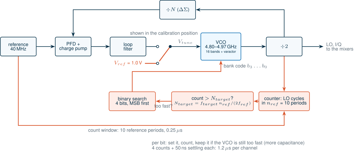
The course synthesizer can count the divide-by-two output that already exists for the mixers (Chapter 13). Over \(n_{ref}\) periods of the 40 MHz reference it counts \(f_{VCO}\,n_{ref}/(2f_{ref})\) cycles, uncertain by one cycle, so its frequency resolution at the VCO is
\[\Delta f_{res} = \frac{2 f_{ref}}{n_{ref}}. \tag{11.16}\]With \(n_{ref}\) = 10 (0.25 µs), \(\Delta f_{res}\) = 8.0 MHz, well below the spacing of the bands, 27.2–39.0 MHz at 1.0 V over all codes and corners. A binary search then sets the four bits from the top down: try a bit, count, and keep it if the VCO is still too fast (more capacitance, lower frequency). Four counts, with 50 ns after each switch for the VCO to settle, take 1.2 µs per channel. Chapter 19 budgets 5 µs, a microsecond per step; BLE, which moves to a new channel at every connection event, can afford either.
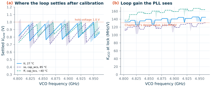
When the loop closes, \(V_{tune}\) moves from the hold voltage to wherever the chosen band reaches the target. The search leaves the target between the chosen band and the next one at the hold voltage, so the loop settles below the hold voltage (or up to \(\Delta f_{res}/K_{VCO}\) above it, from the counter’s uncertainty), within a window of about
\[\Delta V_{tune} \approx \frac{\Delta f_{band} + \Delta f_{res}}{K_{VCO}}. \tag{11.17}\]We ran the search on the transients of Section 11.5, extended to every code from 0.3 to 1.2 V in steps of 0.1 V in all three corners (412 more 20 ns transients): 81 targets in 2 MHz steps across the course band, each with 50 random counter phases. Figure 11.10 shows the result for a hold voltage of 1.0 V. The loop settles between 0.644 and 1.04 V in every corner, using codes 6–11 at the typical corner, 3–8 in the slow corner and 10–15 in the fast corner. That last range ends at code 15: as Section 11.5 found, the fast corner has no band to spare at the bottom of the course band. After calibration, every channel can still drift by at least 17.7 MHz up and 27.0 MHz down before the varactor reaches the end of the simulated range.
The hold voltage is a design choice, and the shape of the tuning curve decides it. A lower hold voltage puts the settled points where the curve is flat: held at 0.8 V, the loop settles between 0.38 and 0.84 V and sees KVCO from 61.9 to 164 MHz/V, a 2.6:1 spread; held at 0.6 or 0.7 V, some channels would need less than 0.3 V, below the simulated grid, where KVCO falls towards 34 MHz/V. Held at 1.0 V, the loop settles on the steep part of the curve, and KVCO stays between 103 and 167 MHz/V over every channel and corner, a spread of 1.63:1 (4.2 dB).
What this means for your design
The loop never sees the VCO’s average KVCO. A loop filter designed for the 96.9 MHz/V mean at code 8 would see 1.1–1.7 times that once the calibration has chosen the code: its unity-gain frequency would rise roughly in proportion, and its phase margin would fall as the crossover approached the filter’s upper pole. Chapter 12 therefore designs for 131 MHz/V, the geometric centre of the calibrated range, so that the loop gain stays within ±2.1 dB at both ends; scaling the charge-pump current with the bank code would be the alternative, but it costs noise (Section 12.2). And choose the hold voltage from the large-signal tuning curve, not the small-signal one: it decides which part of the curve the loop lives on.
Try the calibration. The demo below runs the same search on the simulated tuning curves of all 16 codes. Pick a channel and a corner and watch the four counts set the bits; then lower the hold voltage and see where the loop has to settle, and what KVCO it gets there.
11.9 Other oscillators
The course VCO is one cross-coupled LC oscillator followed by a divider. Four other ways to build an RF oscillator come up often enough that a designer should know when they would win: two oscillators coupled in quadrature, the second harmonic taken from a common node, many oscillators coupled for lower phase noise, and a transmission line in place of the tank.
Quadrature VCOs
The course radio gets its I and Q LO signals by dividing a 4.8 GHz VCO by two (Chapter 13). A quadrature VCO (QVCO) gets them from two LC oscillators that force each other into quadrature [130]. In each core a second, coupling pair shares the tail and injects a current driven by the other core’s outputs: in phase from B to A, inverted from A to B (Figure 11.11). The only steady state both cores accept has them 90° apart. Each core’s coupling current is then in quadrature with its own, so the tank must add a phase shift to keep the loop gain real, which it can do only off resonance:
\[\frac{\Delta\omega}{\omega_0} \approx \frac{m}{2Q}, \tag{11.18}\]with \(m\) the ratio of the coupling pair’s transconductance to the switching pair’s. Off resonance the tank’s impedance is lower, so the amplitude falls, and the coupling devices add noise of their own; Andreani et al. analyse both [131].
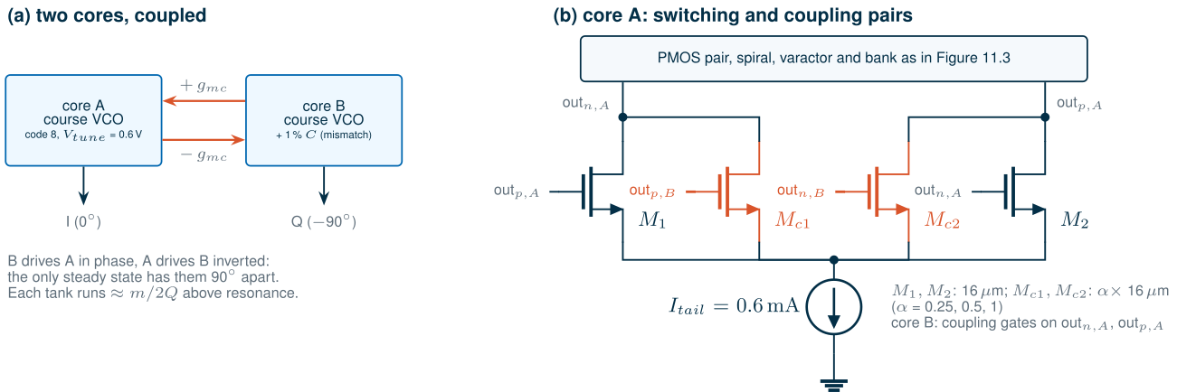
We coupled two copies of the course VCO (code 8, 0.6 V) with coupling pairs a quarter, half and the full width of the switching pair, and ran 120 ns transients (Table 11.4). The coupling devices also load each tank: a single core carrying the same extra devices, wired into its own cross-coupled pair, runs 0.68–2.62 % below the course VCO, so the offsets are measured from that loaded core. With matched cores the QVCO locks at −90.00° for α = 0.25 and 0.5 and runs above the loaded resonance by 0.802 % and 1.43 %, a little below Eq. (11.18)’s 0.84 % and 1.68 % with \(m\) taken equal to α. At α = 0.5 the amplitude falls from 0.784 V to 0.652 V, and the two cores draw 1.55 mW, twice the single VCO.
Table 11.4. Two course VCO cores coupled in quadrature (Figure 11.11; tt, 27 °C, code 8, Vtune = 0.6 V; 120 ns transients, measured over the last 10 ns). Offset: from a single core loaded with the same coupling devices. Mismatch: 5.37 fF (1 % of the tank) across core B.
| Coupling α | Loaded core | QVCO | Offset (Eq. 11.18) | Phase, matched | Phase, 1 % mismatch | Amplitude A, B (1 % mismatch) |
|---|---|---|---|---|---|---|
| 0.25 | 4.835 GHz | 4.874 GHz | +0.802 % (0.84 %) | −90.00° | −65.5° (24.5° error) | 0.753, 0.610 V |
| 0.5 | 4.803 GHz | 4.871 GHz | +1.43 % (1.68 %) | −90.00° | −85.8° (4.24° error) | 0.686, 0.605 V |
| 1 | 4.740 GHz | 4.853 GHz | not settled | −86.2° to −93.8° | −87.9° to −94.4° | 0.684, 0.654 V |
The weakness is mismatch. Add 1 % to one tank’s capacitance and the quadrature error is 24.5° at α = 0.25 and 4.24° at α = 0.5: the weaker the coupling, the more each core follows its own tank, and the amplitudes part as well. Chapter 19 allows 2° of I/Q phase error, which at α = 0.5 asks for tanks matched to about 0.5 %. Stronger coupling is no simple cure: at α = 1 the phase between the cores had not settled after 120 ns, but swung between −86.2° and −93.8° from one 10 ns window to the next. The course radio’s divide-by-two sets its quadrature with flip-flops instead (Chapter 13), at the cost of 2.01 mW and a VCO at twice the frequency; a QVCO needs no divider, but twice the VCO power and a well-matched pair of tanks.
Push-push: the second harmonic at the common node
A differential oscillator’s two outputs carry the fundamental in antiphase and the even harmonics in phase. At a node where the two halves meet, the fundamentals cancel and the second harmonics add: the tail of a cross-coupled pair, or the common mode of its outputs. A push-push oscillator takes its output there and so delivers twice the frequency its tank resonates at [133]. That is attractive where a tank at the output frequency would be hard to build: a 50 GHz LO for Chapter 17’s band from a 25 GHz core, whose varactor has twice the Q it would have at 50 GHz.
The course VCO shows how small that signal is when nobody asks for it. Its 1 pF tail capacitor shorts 2f0, and the tail swings only 5.36 mV at 9.74 GHz; the common mode of the outputs carries 9.13 mV, 32.7 dB below the 392 mV fundamental on each output (the cached transient of Section 11.8). A push-push design does the opposite: it lets the common node swing, often with a resonator tuned to 2f0, and buffers it. Its output is single-ended and weaker than the fundamental, and its phase noise is that of the core plus 6 dB (the phase doubles with the frequency), so it buys frequency, not purity.
Coupled oscillators: phase noise for power
Couple N identical oscillators tightly and they lock to one frequency, while their noise, being uncorrelated, partly averages out: the carrier power grows as N² and the noise power as N, so the phase noise falls by 10 log10N [132]:
\[\mathcal{L}_N(\Delta f) = \mathcal{L}_1(\Delta f) - 10\log_{10}N, \qquad P_N = N P_1. \tag{11.19}\]Two course VCOs would reach about −119.7 dBc/Hz at 1 MHz for 1.53 mW, four about −122.7 dBc/Hz for 3.06 mW. The FoM of Eq. (11.15) does not change: coupling trades power for phase noise one for one, exactly as scaling one oscillator would (half the inductance, twice the capacitance and twice the current, Eq. (11.9)). It is a way to build that larger oscillator from proven cells, not a way to beat the FoM. The course VCO needs neither, with 12.7 dB to spare.
Standing-wave oscillators
At millimetre waves a lumped tank gets awkward: the inductance needed falls to about a hundred picohenries, comparable with the wiring, and the varactor’s Q falls with frequency. A transmission line then becomes the resonator. In a standing-wave oscillator a quarter- or half-wave line carries a standing wave, and gain cells along it cancel its loss; every point oscillates in phase, with an amplitude set by the wave, which also makes the line a clock-distribution network. Andress and Ham taper the line to suit the wave, which raises its Q and its frequency [134]. Chapter 17’s lines (Section 17.4) and Chapter 18’s EM flow are the tools to design one in SG13G2.
Try it · The VCO script
Every number in this chapter comes from
tools/figs/ch11_lc_vco.pyand the netlists of_ch11_vco.py.python3 tools/figs/ch11_lc_vco.pyredraws the figures from the cache;python3 tools/figs/ch11_lc_vco.py <parts> --resimreruns the named parts (isfdev,frozen,dcinj,lstune,afc,qvcoandtrnoise, anddesign_c15ss,tank_c15ss,isfdev_c15ss,frozen_c15ssanddcinj_c15ssfor the slow-corner point;trnoisetakes about an hour,afcabout twenty minutes, the others a few minutes). Five experiments: (1) Make the tail filter’s capacitor four times larger (DESIGN["cfilt"]) and rerunfrozen dcinj --resim: how much lower is the phase noise at 100 kHz, and where does the 1/f³ corner move? (2) Halve the tail current (DESIGN["itail"]) and rerundesign isfdev frozen dcinj --resim: by how much do the amplitude, the phase noise at 1 MHz and the equivalent F change, and does Eq. (11.9) predict the change? (3) Add 10 fF of fixed capacitance (a largercfix) and rerunlstune --resim: how much margin do the slow and fast corners leave at each end of the band now? (4) Inafc_analysis, halven_refto 5 and redraw (no new simulation): how much wider is the settled window of Eq. (11.17), and does every channel still find a band? (5) Add α = 0.75 toQV_ALPHAand rerunqvco --resim: where between the half- and full-width couplings does the quadrature error from 1 % mismatch fall below 2°?
- An LC oscillator is a tank whose loss a negative resistance cancels; a cross-coupled pair gives −2/gm, and the course VCO starts with a margin of 2.6 at 0.6 mA.
- In SG13G2 at 2.4–5 GHz the tank Q (14.9 for the course tank, 15.9 for the FPLL-style tank) is set by the spiral; the capacitor bank is the second loss.
- A complementary pair gives twice the swing per milliampere of an NMOS-only pair; SiGe HBTs give more gm per milliampere and a flicker corner four orders of magnitude lower, at the price of headroom.
- A 4-bit bank and a small varactor cover 4.633–5.224 GHz at the typical corner (transients), and the course band in the slow and fast corners too, with only 1 % to spare below it in the fast corner. The large-signal KVCO, 96.9 MHz/V on average in the middle band, is 10 % below the small-signal estimate and varies by four times across the tuning range.
- The ISF can be measured with small charge impulses in an ngspice transient, at every node of the core, and each transistor’s cyclostationary noise taken from frozen operating points; together (Eq. 11.13) they replace Leeson’s noise factor by a simulation. For the course VCO they give −116.7 dBc/Hz at 1 MHz, an equivalent F of 3.71, inside the usual guess of 2–5 and 12.7 dB below the specification at 0.766 mW. The PMOS pair is the largest contributor. At the bank’s largest code in the slow corner (85 °C, 87.5 % of the swing) the phase noise is only 0.43 dB worse, and the LO still meets −110 dBc/Hz at 1 MHz with 2.8 dB to spare.
- The DC part of an effective ISF, which sets the up-conversion of slow noise, is best measured directly, as the frequency shift of a DC injection. In the course VCO the 1/f³ corner (254 kHz) is set by the thermal noise of the tail’s bias filter resistor through frequency pushing, not by the transistors’ flicker noise (65 kHz).
- A counter on the divide-by-two and a 4-bit binary search pick the bank code in 1.2 µs per channel. Holding Vtune at 1.0 V during the search leaves the loop where KVCO is 103–167 MHz/V over every channel and corner, so Chapter 12 designs its loop for the centre, 131 MHz/V, not for the 96.9 MHz/V average.
- Two coupled cores give quadrature without a divider, but 1 % of tank mismatch costs 4.24° at half-width coupling (24.5° at quarter width); coupling N oscillators trades power for phase noise at a constant FoM, and push-push and standing-wave oscillators reach frequencies a lumped tank cannot.
Further reading
- D. B. Leeson [120]: the two-page paper behind Eq. (11.8).
- A. Hajimiri and T. H. Lee [121]: the impulse sensitivity function, cyclostationary noise and the 1/f³ corner; their companion paper [122] applies it to the differential LC oscillators of this chapter; A. Demir et al. [123] for the rigorous nonlinear theory.
- J. J. Rael and A. A. Abidi [124]: a physical account of where the phase noise of a cross-coupled LC oscillator comes from, and E. Hegazi et al. [125] for the tail filter that removes much of the tail’s contribution.
- D. Ham and A. Hajimiri [126]: optimizing an integrated LC VCO under power and tuning constraints.
- P. Andreani et al. [127] on Colpitts against cross-coupled oscillators, and A. Mazzanti and P. Andreani [128] on class-C VCOs, which reach a better figure of merit than the class-B circuit of this chapter.
- T.-H. Lin and W. J. Kaiser [129]: an early synthesizer that calibrates its VCO’s switched capacitors automatically, the idea behind Section 11.8’s band calibration.
- A. Rofougaran et al. [130] introduced the coupled quadrature LC oscillator of Section 11.9, and P. Andreani et al. [131] analyse its phase noise and phase error; H.-C. Chang et al. [132] derive the 10 log N of coupled oscillators; F. X. Sinnesbichler [133] builds push-push oscillators with SiGe HBTs at millimetre waves; W. F. Andress and D. Ham [134] design standing-wave oscillators on tapered lines.
- B. Razavi, RF Microelectronics [6] (chapter on oscillators) and Design of CMOS Phase-Locked Loops [11]: a textbook treatment of LC VCOs and their design.