Lab 8
Capstone: The Transceiver Budget
The course radio was budgeted in Chapter 5 and designed block by block in Chapters 9–16. This lab puts it back together as Chapter 19 does: the receive cascade from each block's simulated numbers, the synthesizer's phase noise against the interferers it must survive, a bit-error test of the whole receiver, and the transmitter against the spurious-emission rules. It ends with your report: every number against its target, and how it was obtained.
- Compute a receiver’s noise figure, IIP3 and sensitivity from its blocks with Friis’s formula and the cascaded IIP3, and say which block sets each by its share (Eq. 19.1).
- Turn a synthesizer’s phase noise and a receiver’s noise figure into a reciprocal-mixing margin for each interferer.
- Run a behavioural bit-error test of the receiver and compare it with the sensitivity formula.
- Check a transmitter’s harmonics against the ETSI and FCC limits, from a field strength to an equivalent power.
- Write a block-by-block verification report that states, for every number, how it was obtained.
Contents
| Lab 8 at a glance | |
|---|---|
| Goal | The course radio against its budget: receiver NF, IIP3 and sensitivity, the LO against reciprocal mixing, one behavioural BLE test, the transmitter’s harmonics, and a report against Table 5.3. |
| Chapters | Chapter 5 (Table 5.3, Eq. (5.18)); Chapter 19 (Sections 19.1–19.3, Tables 19.1–19.4, Eqs. (19.1) and (19.2)); Chapter 4 for Eqs. (4.11) and (4.12); the block numbers of Chapters 9–16, or of your Labs 4, 5 and 7 |
| Time | 2 × 3 hours: the receiver in the first session, the transmitter and the report in the second |
| Files | tools/labs/lab8/: transceiver_lab.py; it imports tools/figs/_ch19_rx.py (the behavioural receiver), ch19_transceiver.py (the band filter, and its cascade() as a check), ch14_fractional_n.py and ch12_pll_noise.py (the synthesizer), and reads ch04, ch05, ch09–ch14, ch16 and ch19_numbers.json in tools/figs/ |
| Run time | cascade, lo, tx, margins and report under a second each; ber about 13 s; all about 15 s |
No circuit is simulated in this lab. Its inputs are the numbers the block chapters, and your own labs, have already simulated; its work is to combine them correctly and to keep track of where each one came from.
Hand calculation
The receiver of Figure 19.1 has four blocks. Two are designed in the course: the LNA (Chapter 9: gain 17.61 dB, NF 1.17 dB, IIP3 −4.9 dBm) and the I/Q mixer with its TIA (Chapter 10’s final design, with a transistor-level OTA in both TIAs and RF = 223 Ω: +8.05 dB, 11.88 dB, +10.6 dBm). Two keep the allocation of Table 5.3: the band filter with the T/R switch (−2 dB, 2 dB, +40 dBm) and the complex filter with the VGA (+30 dB, 20 dB, +14 dBm).
- Noise figure. Evaluate Friis’s formula (Eq. 4.11) with linear gains and noise factors, \(F = F_1 + (F_2 - 1)/G_1 + (F_3 - 1)/G_1G_2 + (F_4 - 1)/G_1G_2G_3\). Write down the four terms: each divided by the sum is the block’s noise share of Eq. (19.1).
- IIP3. Evaluate \(1/\mathrm{IIP3} = 1/\mathrm{IIP3}_1 + G_1/\mathrm{IIP3}_2 + G_1G_2/\mathrm{IIP3}_3 + G_1G_2G_3/\mathrm{IIP3}_4\) with the IIP3s in milliwatts, and the IIP3 shares.
- Sensitivity. Eq. (4.12) with 1 MHz of noise bandwidth and the 12.3 dB of SNR that GFSK with a discriminator needs for 0.1 % BER (Chapter 4): \(P_{sens} = -174 + 60 + \mathrm{NF} + 12.3\) dBm.
- Reciprocal mixing. Chapter 5’s course case puts the wanted signal at −87 dBm and an interferer of −40 dBm 3 MHz away. With your NF, how much power may the LO’s phase noise mix into the 1 MHz channel, once the thermal noise has taken its share of the 12.3 dB? Which L(3 MHz) does Eq. (5.18) then require?
- The FCC limit. In the restricted bands that hold both harmonics, FCC Part 15 allows a field of 500 µV/m at 3 m [190]. A transmitter of EIRP \(P\) produces \(E = \sqrt{30P}/d\) in free space: which \(P\) is that, in dBm? Which harmonic level in dBc does it require at +10 dBm, and which does ETSI’s −30 dBm require [189]?
- Second order. Eq. (19.2): refer the mixer’s IIP2 to the antenna. With the OTA, Chapter 10 found it no lower than +41.5 dBm (a bound: its IM2 product does not grow with a slope of 2).
Steps, first session: the receiver
Work in tools/labs/lab8. Inside the container, run the commands as shown; from your own computer, put ../common/iic.sh in front of each (Lab 0). Each step prints its results and stores them in lab_numbers.json.
-
The cascade.
cd /foss/designs/rfic-design/tools/labs/lab8
python3 transceiver_lab.py cascade     # from your computer: ../common/iic.sh python3 transceiver_lab.py cascade
The script reads each designed block’s numbers from the JSON file of the chapter that simulated it. Do it once by hand in
python3, to see where each number lives:import json J9 = json.load(open("../../figs/ch09_numbers.json")) J9["design"]["main"]["s21_f0"], J9["design"]["main"]["nf_f0"], J9["hb"]["iip3"] # LNA: 17.61, 1.17, -4.9 J10 = json.load(open("../../figs/ch10_numbers.json")) J10["mix_ota"]["g_db"], J10["mix_ota"]["nf_htm"], J10["mix_ota"]["iip3"][0] # mixer with the OTA: 8.05, 11.88, 10.6 json.load(open("../../figs/ch19_numbers.json"))["assume"]["baseband"] # the assumed blocksSOURCESat the top oftransceiver_lab.pylists every number the lab uses, with its place in the chapter’s file and in your lab’s file.cascade()is the hand calculation in NumPy [31]: the Friis terms, the terms of 1/IIP3 and their cumulative sums give the NF and IIP3 after each block and the shares of Eq. (19.1). The step prints the cascade row by row (Table 19.2), the sensitivity of Eq. (4.12), the same for the budget of Table 5.3, the NF without the band filter, the IIP3 of the RF front end and of the baseband referred to the antenna (the two nonlinearities of the behavioural receiver in step 3), and the IIP2 at the antenna. With SciPy’sbrentq[178] it also finds how far the mixer’s and the baseband’s NF could rise before the system NF reaches the 8 dB of the specification. Last, it calls Chapter 19’s owncascade()on Chapter 19’s blocks: the two codes must agree. -
The LO against reciprocal mixing.
python3 transceiver_lab.py loThe phase noise at the 2.44 GHz LO is Chapter 14’s model of the course synthesizer in its design case,
ch14_fractional_n.budget_design(): Chapter 11’s simulated VCO in Chapter 12’s 400 kHz loop, with the MASH 1-1-1 and the modelled, calibrated DTC. The step prints L(f) at five offsets and the phase error from 10 kHz to 8 MHz, and checks the two lines of Table 5.3. Then it does Hand calculation 4 for every interferer of Chapter 19’s list: the course cases (wanted −87 dBm, interferers at 2, 3 and 27 MHz) and BLE’s own C/I tests (wanted −67 dBm). The requirement depends on the NF of step 1: a noisier receiver leaves less room for the LO. -
One behavioural BLE test: sensitivity.
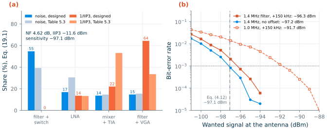
python3 transceiver_lab.py berchain()builds Chapter 19’s behavioural receiver (_ch19_rx.Chain) from this lab’s cascade: thermal noise for the NF of step 1, a saturating third-order nonlinearity for the front end and one for the baseband with the IIP3s of step 1, the synthesizer’s phase noise of step 2, the I/Q errors of the 1 % chip of Chapter 19’s Monte Carlo (−0.219 dB, −1.54°), the assumed band filter, a fourth-order complex Butterworth channel filter at a 1 MHz IF and a 6-bit ADC.sens_curve()sends 100 000 random GFSK bits per point at −101, −100, … dBm until the BER falls below 2 × 10⁻⁵, with Chapter 19’s seeds, and the sensitivity is where the BER crosses 0.1 %. It runs three receivers: Chapter 19’s recommended 1.4 MHz filter with the +150 kHz carrier offset that BLE allows [184], the same filter without offset, and Table 5.3’s 1.0 MHz filter with the offset.--cases bw14_150runs only the first.
Steps, second session: the transmitter and the report
-
The transmitter.
python3 transceiver_lab.py txThe PA is Chapter 16’s off-chip network with both traps, the one of Lab 7. The step prints its drive, PAE, collector efficiency and current at +10 dBm, its headroom to saturation, the power at the antenna if the transmitter shares the 2 dB band filter and T/R switch with the receiver, and the DC power of the transmit chain: the PA, Chapter 11’s VCO and Chapter 13’s divide-by-two and prescaler. Then the regulations: ETSI EN 300 328’s −30 dBm from 1 to 12.75 GHz, and the FCC limit in the restricted bands, which
fcc_limit_dbm()converts from the field strength as in Hand calculation 5. The harmonics are counted at the antenna with no help from the band filter, as Chapter 19 does. For comparison it lists the two harmonics of Chapter 16’s other off-chip networks, without traps and with the 3f0 trap alone. -
Every number against its target.
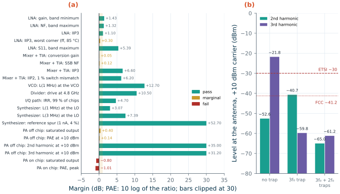
python3 transceiver_lab.py marginsThis is Table 19.1 rebuilt: 22 numbers of the designed blocks (the LNA, mixer, VCO, divider, I/Q path, synthesizer and PA) and the three receiver numbers of step 1, each with its target, its margin in dB (for PAE, 10 log of the ratio), a status (fail below 0 dB, marginal below 1 dB) and how it was obtained. The synthesizer’s two phase-noise numbers come from step 2’s run of Chapter 14’s model; the others from the chapters’ files.
-
The report.
python3 transceiver_lab.py allruns steps 1–5, draws Figure L8.1 and Figure L8.2 intoout/, and writesout/lab8_report.md: the template of the next section with your numbers filled in and the paragraphs left for you.python3 transceiver_lab.py reportrewrites it without rerunning the bit-error test. -
Your own numbers. Rerun with
--source labs: the LNA’s, mixer’s and PA’s numbers now come from thelab_numbers.jsonof your Labs 4, 5 and 7 (the on-chip PA from Lab 7’s--net chiprun), and the “how obtained” column names the lab. The results go intolab_numbers.jsonundercascade_labs,margins_labsand so on, next to those from the chapters’ files. Lab 5 simulates Chapter 10’s behavioural op-amp, not the transistor-level OTA that Chapter 19 uses, so the mixer’s numbers, and the receiver’s, differ a little from the chapter’s (see the Checkpoint).
The capstone report
Your deliverable is a short report, at most two pages, that a reviewer can check line by line. Its core is the table against Table 5.3 and the course radio, and its most important column is the last but one: how each number was obtained, so that the reader knows which margins rest on a simulation, which on a hand analysis, a behavioural model or an assumption, and which you took from a chapter instead of producing yourself. out/lab8_report.md gives you this template filled with your numbers; write the parts in angle brackets.
# The course transceiver against its budget
Author · date · image (IIC-OSIC-TOOLS 2026.10) · block numbers from (chapters / your labs)

## 1. Summary
<Does the radio meet the course specification? Which numbers are marginal or fail?
 Which single number would you verify next, and why?>

## 2. Receiver blocks against Table 5.3
| Block | Table 5.3: gain / NF / IIP3 | Designed: gain / NF / IIP3 | How obtained | Source |
|---|---|---|---|---|
| Band filter + T/R switch | −2 dB / 2 dB / +40 dBm | ... | assumed: Table 5.3 allocation | — |
| LNA | +16 dB / 2.5 dB / −6 dBm | ... | ngspice sp; sp noise; Xyce two-tone HB | Lab 4 or Ch. 9 |
| I/Q mixer + TIA | +8 dB / 12 dB / +4 dBm | ... | Xyce transient; periodic small-signal; Xyce two-tone (Ch. 10: transistor-level OTA; Lab 5: behavioural op-amp) | Lab 5 or Ch. 10 |
| Complex filter + VGA | +30 dB / 20 dB / +14 dBm | ... | assumed: Table 5.3 allocation | — |
| Receiver | +52 dB / 6.06 dB / −12.7 dBm; −95.6 dBm | ... | Friis, cascaded IIP3, Eq. (4.12) | Lab 8 |
Noise and IIP3 shares (Eq. 19.1). <Which block would you improve first, and what would it cost?>

## 3. Every designed number against its target
| Block | Item | Target | Value | Margin | Status | How obtained | Source |
|---|---|---|---|---|---|---|---|
| ... one row per number: LNA, mixer, VCO, divider, I/Q path, synthesizer, PA, receiver ... |

## 4. The LO
L(1 MHz), L(3 MHz) at the LO; the reciprocal-mixing requirement and margin for each interferer.

## 5. One behavioural BLE test
Sensitivity at 0.1 % BER with the 1.4 MHz filter and a +150 kHz offset, against Eq. (4.12) and BLE's −70 dBm.

## 6. The transmitter
P_out, PAE, headroom; DC power; harmonics at the antenna against ETSI and FCC.

## 7. What is not verified
<Every number above that no simulation of yours produced (assumed, hand analysis, behavioural model,
 taken from a chapter), and the one that sits closest to its limit.>
Be specific in the “how obtained” column: not “simulated” but “ngspice sp with noise, tt, 27 °C, Lab 4” or “Xyce two-tone harmonic balance, ff, 85 °C”; not “from the chapter” but “Chapter 11, ISF with frozen noise sources, not rerun”. Two numbers obtained differently deserve two rows.
Checkpoint
Table L8.1. Lab 8, the receiver (block numbers from the chapters' JSON files unless stated; tt, 27 °C; phase noise at the 2.44 GHz LO). Tolerance: ±1 in the last digit shown, except where stated.
| Quantity | Lab 8 | Chapter 19 |
|---|---|---|
| Hand calculation: Friis terms; NF | 1.585 + 0.490 + 0.396 + 0.426 = 2.897; 4.62 dB | 4.62 dB |
| Hand calculation: IIP3; sensitivity | −11.6 dBm; −97.1 dBm | −11.6 dBm; −97.1 dBm |
| Hand calculation: room for reciprocal mixing at −87 dBm; L(3 MHz) required | −99.7 dBm; −119.7 dBc/Hz | −99.7 dBm; −119.7 dBc/Hz |
| Hand calculation: FCC limit as EIRP; harmonics required at +10 dBm (FCC, ETSI); IIP2 at the antenna | −41.2 dBm; −51.2, −40 dBc; +25.9 dBm | −41.2 dBm; +25.9 dBm |
| Cascade: gain, NF, IIP3 | 53.66 dB, 4.62 dB, −11.6 dBm | 53.66 dB, 4.62 dB, −11.6 dBm (Table 19.2) |
| Cascade NF after each block | 2.00, 3.17, 3.93, 4.62 dB | 2.00, 3.17, 3.93, 4.62 dB |
| Cascade IIP3 after each block | +40.0, −2.9, −7.1, −11.6 dBm | +40.0, −2.9, −7.1, −11.6 dBm |
| Noise shares: filter, LNA, mixer, baseband | 54.7, 16.9, 13.7, 14.7 % | 54.7, 16.9, 13.7, 14.7 % |
| IIP3 shares | 0.0, 13.6, 22.1, 64.4 % | 0, 13.6, 22.1, 64.4 % |
| Sensitivity (Eq. 4.12); margin to −90 and to −70 dBm | −97.1 dBm; 7.1, 27.1 dB | −97.1 dBm; 7.1, 27.1 dB |
| Budget of Table 5.3: NF, IIP3, sensitivity | 6.06 dB, −12.7 dBm, −95.6 dBm | 6.06 dB, −12.7 dBm, −95.6 dBm |
| NF without the band filter; IIP3 of the front end; of the baseband at the antenna | 2.62 dB; −7.1 dBm; −9.7 dBm | 2.62 dB; −7.1 dBm; −9.7 dBm |
| Mixer NF, baseband NF that would give a system NF of 8 dB | 21.4, 29.5 dB | 21.4, 29.5 dB |
| IIP2 at the antenna; required; margin | +25.9 dBm; +21.3 dBm; 4.6 dB | +25.9 dBm; +21.3 dBm; 4.6 dB |
| L at 100 kHz, 1 MHz, 2 MHz, 3 MHz, 10 MHz | −104.2, −112.7, −121.4, −126.9, −141.5 dBc/Hz | −104.2, −112.7, −121.4, −126.9, −141.5 dBc/Hz |
| Phase error, 10 kHz–8 MHz | 0.41° | 0.41° |
| Reciprocal-mixing margins: 2, 3, 27 MHz (course); 2, 3 MHz (BLE C/I) | 11.6, 7.2, 25.8; 32.1, 27.6 dB | 11.6, 7.2, 25.8; 32.1, 27.6 dB |
| BER sensitivity: 1.4 MHz filter, +150 kHz offset (±0.2 dB) | −96.3 dBm | −96.3 dBm |
| BER sensitivity: 1.4 MHz, no offset; 1.0 MHz, +150 kHz (±0.2 dB) | −97.2 dBm; −91.7 dBm | −97.2 dBm; −91.7 dBm |
With --source labs (Labs 4 and 5 as shipped; Lab 5’s mixer has the behavioural op-amp): NF, IIP3, sensitivity; IIP2 at the antenna; BER sensitivity, 1.4 MHz filter, +150 kHz |
4.54 dB, −11.7 dBm, −97.2 dBm; +39.5 dBm; −96.4 dBm | behavioural op-amp (Section 19.2): 4.54 dB, −11.7 dBm, −97.2 dBm; +40.4 dBm |
Table L8.2. Lab 8, the transmitter and the margins (PA with Chapter 16's off-chip network and both traps, VPA = 2.0 V, +10 dBm). Tolerance: ±1 in the last digit shown.
| Quantity | Lab 8 | Chapter 19 |
|---|---|---|
| Drive; PAE; collector efficiency; PA current | −2.2 dBm (0.60 mW); 31.0 %; 33.7 %; 14.9 mA | −2.2 dBm (0.60 mW); 31.0 %; 33.7 %; 14.9 mA (Table 19.4) |
| Saturated output; headroom; at the antenna through 2 dB; PA output needed for +10 dBm there | 10.4 dBm; 0.4 dB; +8.0 dBm; +12.0 dBm | 10.4 dBm; 0.4 dB; +8.0 dBm; +12.0 dBm |
| DC power PA + VCO + divide-by-two + prescaler; +10 dBm as a fraction of it | 29.8 + 0.77 + 2.01 + 0.18 = 32.8 mW; 30.5 % | 32.8 mW; 30.5 % |
| 2nd harmonic at the antenna; ETSI, FCC margin | −65.0 dBm; 35.0, 23.8 dB | −65.0 dBm; 35.0, 23.8 dB |
| 3rd harmonic at the antenna; ETSI, FCC margin | −61.2 dBm; 31.2, 20.0 dB | −61.2 dBm; 31.2, 20.0 dB |
| Without traps; with the 3f0 trap alone: H2, H3 at the antenna | −52.6, −21.8 dBm; −40.7, −59.8 dBm | −52.6, −21.8 dBm; H2 0.5 dB above the FCC limit |
| Block numbers; fail; marginal | 22; 2; 5 | 22; 2; 5 (Section 19.1) |
| The five marginal margins: mixer gain, mixer NF, PA PAE, LNA IIP3 (ff, 85 °C), PA Psat | +0.05, +0.12, +0.14, +0.30, +0.40 dB | +0.05, +0.12, +0.14, +0.3, +0.4 dB (Table 19.1) |
With --source labs (Labs 4, 5 and 7 as shipped): fail; marginal; mixer gain, NF margins; PA Psat, PAE |
2; 5; +0.02, +0.75 dB; 10.37 dBm, 31.0 % |
Every number reproduces Chapter 19 to the digits shown, the bit-error results included: the behavioural receiver runs with Chapter 19’s seeds and bit counts, so in the same image it gives the same counts. A different NumPy release could change the random streams, which moves a sensitivity by a few tenths of a decibel; hence the wider tolerance.
With --source labs the receiver no longer reproduces Chapter 19, because the mixers differ. Chapter 19 uses Chapter 10’s final mixer, with a transistor-level OTA in both TIAs and RF = 223 Ω; Lab 5 simulates Chapter 10’s behavioural op-amp at 220 Ω, and gives +8.02 dB, 11.25 dB, +9.99 dBm and an IIP2 of +55.2 dBm at −4 dBm per tone. That mixer is 0.63 dB quieter, so the receiver’s NF is 0.08 dB lower (4.54 against 4.62 dB), its sensitivities 0.1–0.2 dB better (−97.2 against −97.1 dBm by Eq. (4.12); −96.4, −97.3 and −91.9 dBm against −96.3, −97.2 and −91.7 dBm in the three bit-error tests), and its IIP2 at the antenna +39.5 dBm instead of the chapter’s bound of +25.9 dBm. These match Chapter 19’s comparison with the behavioural op-amp (Section 19.2: 4.54 dB, −11.7 dBm, −97.2 dBm, and +40.4 dBm from Chapter 10’s +56.0 dBm, within Lab 5’s ±1 dB for this transient number). The Labs 4 and 7 numbers change the results only in the last digit, and the margins keep 2 failures and 5 marginal numbers, with the mixer’s gain and NF at +0.02 and +0.75 dB instead of +0.05 and +0.12 dB.
Questions
- The band filter and T/R switch take 55 % of the noise and the designed LNA only 17 %. Which buys more sensitivity: 0.5 dB less loss in front of the LNA, or an LNA with 0.5 dB less NF? Check your answer with
--filter-loss 1.5. - The designed LNA has 1.6 dB more gain than its allocation. What did that do to the system NF, and what to the IIP3 shares? Would you take some of that gain back, and from which block’s specification?
- Eq. (4.12) and the behavioural receiver agree within 0.1 dB without a carrier offset (−97.1 and −97.2 dBm). Where do the 0.9 dB go with +150 kHz, and why does the 1.0 MHz filter lose 5 dB where the 1.4 MHz filter loses less than 1 dB?
- The reciprocal-mixing requirement at 3 MHz depends on the receiver’s NF. If the NF rose to the specification’s 8 dB, which L(3 MHz) would the course case require? Would the synthesizer still pass?
- Chapter 19 counts the 2 dB of the band filter and switch against the transmitter’s output power but gives the harmonics no credit for the filter’s rejection. Why is that the right way round for a sign-off?
- Of the five marginal numbers, which would you verify next, by which simulation or measurement, and why that one? (Chapter 19’s “What this means for your design” is a hint, not the answer.)
Extension
The phone. Section 19.6 puts the course radio into a smartphone, where a diplexer, a switch and a coexistence filter add up to 2.6 dB of loss in front of the LNA instead of 2 dB. Run python3 transceiver_lab.py cascade ber --filter-loss 2.6 --cases bw14_150 and compare the NF and the Eq. (4.12) sensitivity with Chapter 19’s 5.22 dB and −96.5 dBm. How much of the extra 0.6 dB of loss reaches the behavioural sensitivity?
A corner. The cascade above is typical. Lab 4 stored the LNA at ff, 85 °C as well (ff85 in its lab_numbers.json). Change the three LNA lines of SOURCES to read ff85/s21_f0, ff85/nf_f0 and ff85/iip3, run cascade ber --source labs, and compare with Chapter 19’s corner case (4.94 dB, −96.8 dBm, −11.2 dBm, which combined the worst gain, NF and IIP3 of nine corners); --source labs also takes Lab 5’s behavioural mixer, which lowers the NF by about 0.08 dB against the chapter’s. Which other block would you have to simulate at the same corner before the result means anything?