Chapter 13
Frequency Dividers
A synthesizer is only as fast as its first divider: that circuit runs at the VCO frequency, burns most of the divider chain's power, makes the receiver's quadrature LO, and adds its own noise to every edge it passes on. This chapter designs the course synthesizer's divider chain in SG13G2, from a current-mode-logic divide-by-two at 4.8 GHz, through a TSPC dual-modulus prescaler, to a pulse-swallow counter written in Verilog, and looks at the SiGe and injection-locked dividers that take over at millimetre waves.
- State what a divider must do in a synthesizer, and why its first stage, at the VCO frequency, sets the power, speed and noise of the chain.
- Design a CML latch and a master–slave divide-by-two with quadrature outputs, read its input sensitivity curve, and explain its self-oscillation frequency.
- Compare CML, ECL (SiGe) and TSPC dividers in speed and power, and place each in the divider chain.
- Design a dual-modulus prescaler and pulse-swallow counter for a given division range, and verify it in a mixed transistor-level and Verilog simulation.
- Explain injection-locked and regenerative dividers, estimate their lock range, and estimate a divider’s additive jitter and how it enters the PLL.
Contents
13.1 What a divider must do
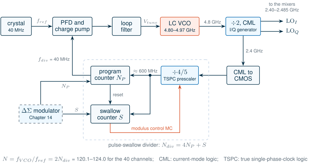
The PLL chapter of The Art of Analog IC Design treated the feedback divider as a behavioural block: a digital model that divides by ten, with no delay, power or noise. In a radio synthesizer the divider is a real circuit, and its first stage is one of the hardest in the chip: it must run at the VCO frequency. Figure 13.1 shows the course synthesizer. The LC VCO of Chapter 11 runs at 4.80–4.97 GHz; a divide-by-two turns it into the quadrature LO at 2.40–2.485 GHz for the mixers of Chapter 10; the same signal continues through a programmable divider to the phase-frequency detector, where it meets the 40 MHz crystal reference. The total division ratio is \(N = f_{VCO}/f_{ref}\) = 120.1–124.0 for the 40 channels of the course radio, fractional, with the fraction supplied by the delta-sigma modulator of Chapter 14.
A divider divides the phase as well as the frequency. If the input is \(\cos[\omega t + \phi_{in}(t)]\), an ideal divide-by-\(N\) produces a square wave whose edges sit at the same instants as every \(N\)th input edge, so its phase is
Key equation · Phase and phase noise through a divider
\[\phi_{out}(t) = \frac{\phi_{in}(t)}{N}, \qquad \mathcal{L}_{out}(\Delta f) = \mathcal{L}_{in}(\Delta f) - 20\log_{10}N. \tag{13.1}\]A timing error of an input edge is passed on unchanged, but it is now a smaller fraction of a longer period. Dividing by two lowers the phase noise by 6.0 dB, which is why the course VCO may be 6 dB noisier than the LO it makes (Chapter 5).
A real divider only approaches Eq. (13.1): it adds noise of its own (Section 13.6). Its other duties make a list of specifications [6, 11]:
- Speed. The first stage must toggle at the highest VCO frequency in every process corner, with margin. Every later stage runs at most half as fast.
- Sensitivity. It must divide correctly with the amplitude the VCO, or a buffer, gives it.
- Power. The dynamic power of logic grows with frequency, so the first stage dominates the chain’s consumption.
- Quadrature accuracy. In the course radio the divide-by-two also makes the I and Q LO signals. Chapter 5 allots 2° of phase error to the whole I/Q path.
- Division range. The programmable part must reach every ratio the fractional-N modulator asks for, including the ones its dither adds (Section 13.4).
- Noise. Within the loop bandwidth, the noise of the divider’s output is multiplied by \(N\) at the VCO, just like the reference’s.
The answer, in Figure 13.1 and in most synthesizers, is a chain of logic families. Current-mode logic, with its small swing and constant current, handles the VCO frequency. After the first divide-by-two, dynamic CMOS logic does the same job with a fraction of the power. Below a few hundred megahertz, ordinary static CMOS logic, synthesized from a hardware description, counts.
13.2 Static CML dividers
The CML latch
A divide-by-two is a flip-flop that toggles, and a flip-flop is two latches. In current-mode logic (CML) a latch steers a current between two load resistors (Figure 13.2a). While the clock CK is high, \(M_5\) conducts and the track pair \(M_1\)–\(M_2\) copies the differential input \(D\) to the output \(Q\). While CK is low, \(M_6\) conducts instead and the cross-coupled latch pair \(M_3\)–\(M_4\) holds the last value. Because the current only moves from one side to the other, the supply current is constant, and the outputs swing by
\[\Delta V = I_T R_L \tag{13.2}\]around \(V_{DD} - \Delta V/2\), where \(I_T\) is the current that the clock pair steers. The swing must be large enough to switch the next latch’s pairs completely, and small enough to keep its transistors out of the triode region.
The latch can only hold a state, and the divider can only regenerate a full swing from the small signal it samples, if the cross-coupled pair has a loop gain above one around its balanced point, where each transistor carries \(I_T/2\) [6]:
Key equation · Gain of a CML latch
\[A_0 = g_mR_L = \frac{g_m}{I_D}\,\frac{\Delta V}{2} > 1, \qquad \tau_{reg} = \frac{C_L}{g_m - 1/R_L}. \tag{13.3}\]\(C_L\) is the capacitance of an output node and \(\tau_{reg}\) the time constant with which the latch regenerates a small difference. For a given swing, the gain depends only on \(g_m/I_D\): a latch biased for speed at a low \(g_m/I_D\) needs a large swing.
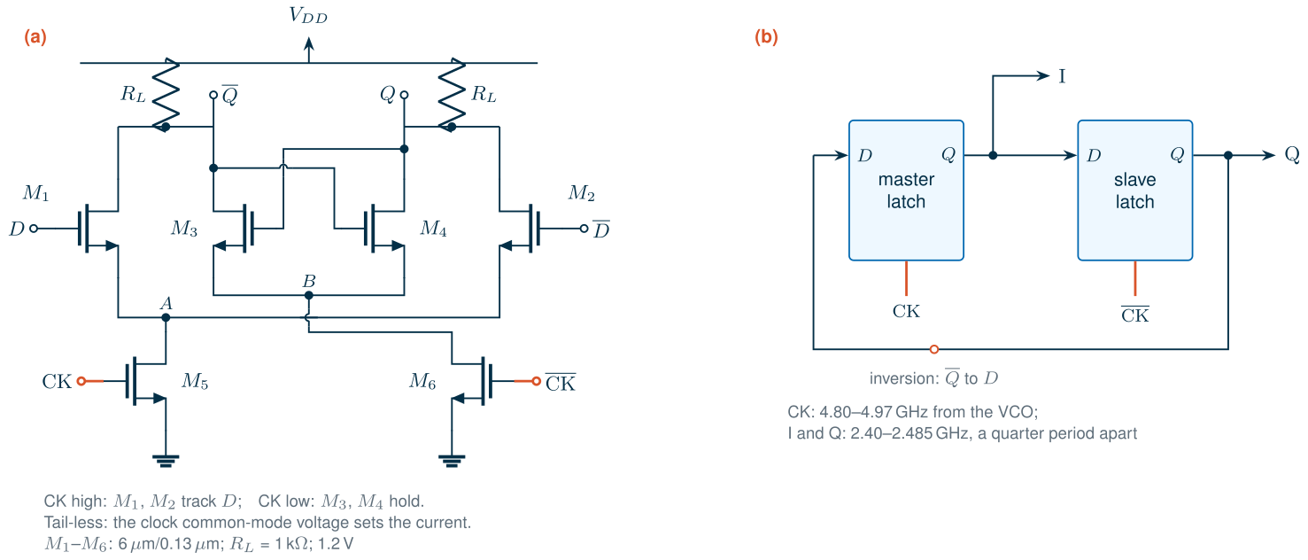
Headroom at 1.2 V. The textbook latch has a tail current source under \(M_5\)–\(M_6\). At 1.2 V, three stacked transistors plus a load resistor leave the tail device too little voltage to be a current source and still give the track and latch pairs a swing that satisfies Eq. (13.3). The course divider therefore drops the tail (Figure 13.2a): the sources of the clock pair go to ground, and the clock’s common-mode voltage \(V_{CM}\), set through AC coupling from the VCO, fixes the current, much like the gate bias of a class-AB stage. The price is that the current now depends on the clock amplitude and common mode, which a replica bias circuit must control in a product.
The master–slave divide-by-two and its quadrature outputs
Two latches in a loop with an inversion, one clocked by CK and the other by \(\overline{\mathrm{CK}}\), make a divide-by-two (Figure 13.2b). The master copies the inverted output of the slave while CK is high; the slave copies the master while CK is low. Each output therefore changes once per input period, and the master’s output changes on the rising edges of CK while the slave’s changes on the falling edges: the two outputs are square waves at half the input frequency, a quarter of their period apart. That quarter period is 90° at the output frequency, so the divider delivers I and Q without any phase-shift network. This is why the course VCO runs at twice the LO frequency.
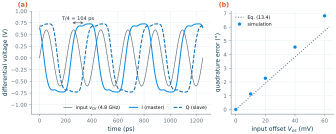
The course divider uses 6 µm/0.13 µm lv nMOS devices for all six transistors of each latch, \(R_L\) = 1 kΩ, \(V_{CM}\) = 0.75 V and a 10 fF load on every output for the LO buffers that follow. Figure 13.3a shows it at 4.80 GHz with a 0.3 V (peak, each side) sine input: the outputs run at 2.400 GHz with a differential swing of ±0.728 V, and Q lags I by a quarter period to within 0.00015°, the numerical floor of the simulation. The divider draws 1.67 mA, 2.01 mW from 1.2 V.
Worked example 13.1 · Swing and gain of the course latch
Each latch carries half of the 1.67 mA, \(I_T\) = 0.835 mA. Eq. (13.2) with \(R_L\) = 1 kΩ predicts a swing of 0.835 V if the clock pair steered all of it; the simulation gives 0.728 V, because a sine clock leaves both clock transistors conducting for part of each period.
At the balanced point of the track pair (CK at its peak, equal inputs), the operating point gives each transistor 0.287 mA, 0.048 mA/µm, with \(g_m/I_D\) = 7.49 V⁻¹: \(g_mR_L\) = 2.15, or 1.79 once the transistors’ own output conductance is counted. The cross-coupled pair in hold mode reaches 2.42 (1.94). Both clear the limit of one with margin; at the measured swing, Eq. (13.3) would accept any \(g_m/I_D\) above \(2/\Delta V\) = 2.75 V⁻¹ for a gain of one.
Chapter 6 found the SG13G2 nMOS fastest at 0.19–0.34 mA/µm (peak \(f_{max}\) and \(f_T\) at \(V_{DS}\) = 0.6 V), where \(g_m/I_D\) is only 3.7–2.3 V⁻¹. By Eq. (13.3) a latch biased there would need a swing of 1.1–1.7 V for a gain of two, impossible at 1.2 V; the course latch trades some of the device’s speed for gain by running at a low current density.
Quadrature error. The 90° depends on the input’s duty cycle: the Q edges follow the falling input edges, so a duty cycle \(D\) puts Q at \(180°\cdot D\) behind I instead of 90°. A sine input of amplitude \(A\) on each side with a differential offset \(V_{os}\) crosses zero early on one edge and late on the other, and the quadrature error becomes
Key equation · Quadrature error from an input offset
\[\Delta\phi_{IQ} = \arcsin\frac{V_{os}}{2A} \approx \frac{V_{os}}{2A}\ \ \mathrm{rad}. \tag{13.4}\]The offset counts against the differential amplitude \(2A\): a large VCO swing makes the I/Q phase robust.
Figure 13.3b compares Eq. (13.4) with the simulation. The divider is a little more sensitive than the equation, 0.114° per millivolt against 0.0955°, because in a tail-less latch the offset also shifts the currents of the two latches and so their delays. One degree of quadrature error, half of Chapter 5’s allocation, corresponds to 8.8 mV of offset at 0.3 V of drive. Mismatch inside the latches matters much less: a 1 % error in one of the slave’s load resistors moves Q by 0.086°, and 5 mV of offset on one of its track transistors by 0.093°, against 0.57° for the same 5 mV at the clock input. The track pair is overdriven by the other latch’s full swing, while the clock pair sees the slowly crossing sine. The duty cycle of the clock, set by the VCO buffer and the matching of the clock pair, decides the I/Q accuracy; at 4.97 GHz, the top of the band, the ideal divider is still exact (0.00035°).
The sensitivity curve and the self-oscillation frequency
With its input clock held at the common-mode voltage, a CML divider is a ring of two differential stages with an inversion: it oscillates. Lee and Razavi pointed out that a CML divider is best understood as such a ring oscillator, injection-locked by the clock [143]. Its free-running, or self-oscillation, frequency \(f_{so}\) is set by the delay of the latches; one oscillation period takes four latch transitions,
\[f_{so} = \frac{1}{4\,t_d}, \tag{13.5}\]with \(t_d\) the delay of one latch. Driven at \(2f_{so}\), the divider only has to be nudged into step and divides with a tiny input. Away from \(2f_{so}\) the clock must force it, and the further away, the larger the amplitude it needs. The input sensitivity curve, the minimum input amplitude against frequency, is therefore a V with its tip near \(2f_{so}\) [143, 11].
Figure 13.4a shows the curves of three designs, from a grid of 45 transients (one per frequency, with ten dividers at ten amplitudes in each). The three designs differ only in their current: the widths double and the load resistors halve from one to the next, so the swing and the self-loading \(R_LC_{dev}\) stay the same, and only the fixed 10 fF load sees the extra current. The nominal design self-oscillates at 4.46 GHz (Eq. 13.5: \(t_d\) = 56.1 ps) and divides with 10 mV, the smallest amplitude tested, at 9 GHz, close to \(2f_{so}\); at the VCO’s 4.8 GHz it needs 100 mV, and its last correct frequency at 0.4 V of drive is 14 GHz. The low-power design (3.48 GHz self-oscillation) has its tip at 7 GHz and stops at 11 GHz; the fast design (5.45 GHz) has its tip at 11 GHz and still divides at 18 GHz with 0.4 V.
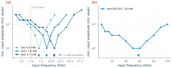
At low frequencies the curves rise again. A slow sine spends a long time near its zero crossing, where both clock transistors conduct, and during that time the divider free-runs and can make extra transitions. A square-wave clock, with fast edges, removes this lower limit: a static CML divider works down to DC, unlike the dynamic dividers of Section 13.3.
Table 13.1. The three CML designs at 4.80 GHz (0.3 V peak input) and the HBT version. Simulated, typical models, 27 °C. Rise time: 20–80 % of the differential output.
| low | nom (course) | fast | npn13G2 ECL | |
|---|---|---|---|---|
| Devices, RL | 3 µm, 2 kΩ | 6 µm, 1 kΩ | 12 µm, 500 Ω | 1 emitter, 150 Ω |
| Supply, power | 1.2 V, 0.98 mW | 1.2 V, 2.01 mW | 1.2 V, 3.97 mW | 2.5 V, 10.0 mW |
| Swing (differential peak) | 0.719 V | 0.728 V | 0.727 V | 0.3 V (design) |
| Output rise time | 52.7 ps | 42.1 ps | 36.6 ps | |
| Self-oscillation fso | 3.48 GHz | 4.46 GHz | 5.45 GHz | 29 GHz |
| Min. input at 4.8 GHz | 75 mV | 100 mV | 150 mV | 100 mV at 5 GHz |
| Max. input frequency (0.4 V drive) | 11 GHz | 14 GHz | ≥ 18 GHz | 100 GHz |
What this means for your design
More current makes a CML divider faster, but at the course’s 4.8 GHz the low-power design is the most sensitive of the three, because its \(2f_{so}\) lies closest to the operating band. Place the band on the low-frequency slope of the V, below \(2f_{so}\), with enough margin that a slow corner, which lowers \(f_{so}\), does not push the tip below the band. The course uses the nominal design: it needs 100 mV where the VCO buffer gives several hundred, toggles to 14 GHz, almost three times the band, and its faster edges (42.1 ps against 52.7 ps) drive the LO buffers more firmly and add less jitter (Section 13.6), for 1.03 mW more than the low-power design.
What SiGe buys: an ECL divider
The same topology built from npn13G2 HBTs is the classic emitter-coupled logic (ECL) divider of high-speed bipolar circuits [140, 10]. Bipolar pairs switch completely with a much smaller input than MOS pairs, so the swing drops to 0.3 V (\(R_L\) = 150 Ω), and with one emitter per transistor and 2 mA per latch, the device that carries the whole current runs at 31.7 mA/µm², just below the current density of peak \(f_T\) that Chapter 6 found (42.8 mA/µm²). Two stacked base–emitter junctions and a tail current source need 2.5 V; each transistor still sees less than its \(BV_{CEO}\) of 1.6 V. The tail is an ideal current source in this simulation.
Figure 13.4b shows the result: a self-oscillation frequency of 29 GHz, a sensitivity tip at 50–60 GHz (10 mV, the smallest amplitude tested), and correct division up to 100 GHz with 100 mV of drive, for 10.0 mW. That is 7.1 times the maximum frequency of the nominal CMOS design for 5.0 times its power. For the 2.4 GHz radio the HBT divider would be a waste of power. A 50 GHz synthesizer, the kind a millimetre-wave radio around the amplifier of Chapter 17 would need, could divide its VCO directly with it: in SG13G2 it is the only static divider that works there.
13.3 TSPC and dynamic dividers
After the first divide-by-two, the signal is at 2.4 GHz and the quadrature outputs are no longer needed for the feedback path. Here dynamic CMOS logic beats CML: it draws power only when it switches. The classic circuit is the true single-phase-clock (TSPC) flip-flop of Yuan and Svensson (Figure 13.5a) [138]. Its first stage is a p-type latch that passes the inverted input to node \(a\) while CK is low. The second stage precharges node \(b\) high while CK is low and, when CK rises, discharges it if \(a\) is high. The third stage, an n-type latch, inverts \(b\) to the output while CK is high and holds it while CK is low. The output therefore takes the inverted value of \(D\) at each rising edge; with \(\overline{Q}\) connected back to \(D\), the flip-flop toggles and divides by two. All nine transistors see the same clock phase, so no complementary clock is needed, and the circuit uses no static current.
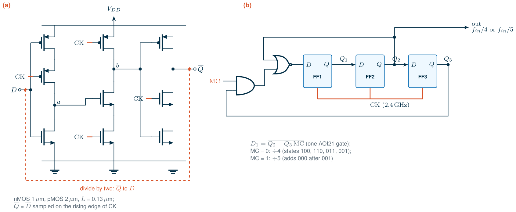
The charge on nodes \(a\) and \(b\) and on the output is held on capacitance alone during part of each cycle, so leakage sets a minimum clock frequency (not simulated here); it is no limit at 2.4 GHz, but it rules TSPC out of slow counters. Its dynamic power is that of a switched capacitance,
\[P = C_{eff}V_{DD}^2f, \tag{13.6}\]where \(C_{eff}\) lumps the switched capacitances and the short-circuit current per cycle.
Figure 13.6a shows the maximum input frequency of a TSPC divide-by-two (nMOS 1 µm, pMOS 2 µm, an output inverter and 2 fF load), driven by a rail-to-rail trapezoidal clock, against the supply. At 1.2 V it divides up to 7 GHz, and from 0.8 to 1.4 V its range grows from 2 to 10 GHz, because the transistors’ current, and so the speed of every node, rises with \(V_{DD} - V_{TH}\). Figure 13.6b confirms Eq. (13.6): the power at 1.2 V grows linearly with frequency, with a slope of \(C_{eff}\) = 14.4 fF, on top of 17 µW that the short-circuit current draws during the slow clock edges (each lasts a quarter period, so it costs about the same power at every frequency). At 2.4 GHz the divider draws 63.6 µW, 32 times less than the CML divide-by-two at twice the frequency. Neither number includes the circuit that drives the clock.
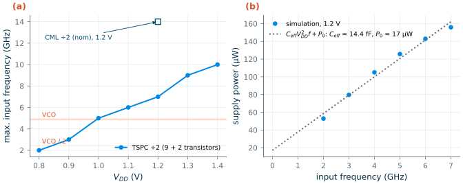
TSPC could even replace the CML divider at 4.8 GHz, where it would draw 122 µW instead of 2.01 mW. But its 7 GHz at 1.2 V is only 1.4 times the top of the VCO band, little margin for slow corners and high temperature (not simulated here), and it would need a rail-to-rail clock, which the VCO does not provide without a power-hungry buffer, and its single-ended outputs are not in quadrature. In the course chain TSPC takes over after the first divide-by-two, where its speed has margin and its power is negligible; a CML-to-CMOS converter, a self-biased inverter or a differential-to-single-ended amplifier, sits between the two.
13.4 Dual-modulus prescalers and pulse-swallow counters
The division ratios the course needs
The programmable divider sees the divide-by-two’s 2.40–2.485 GHz and must divide it by \(N_{div} = N/2\) = 60.05–62.00 for the 40 channels. The fraction comes from a delta-sigma modulator that dithers the integer ratio from one reference cycle to the next (Chapter 14). A third-order MASH modulator, a common choice, adds between −3 and +4 to the integer part, so the divider must reach every integer from 57 to 66; we design for 56–67, which leaves a step of margin at each end for whatever modulator Chapter 14 settles on.
A programmable counter that runs at 2.4 GHz and reloads a new ratio every cycle would be large and power-hungry. The dual-modulus prescaler avoids it [139, 6]: a small, fast divider that divides by \(P\) or \(P+1\) under a modulus-control input MC, followed by two slower counters. A program counter counts \(N_P\) prescaler cycles and then restarts the frame; a swallow counter holds MC high, and the prescaler at \(P + 1\), for the first \(S\) of them. One frame lasts \(S(P+1) + (N_P - S)P\) input cycles:
Key equation · Pulse-swallow divider
\[N = P\,N_P + S, \qquad 0 \le S \le P - 1,\quad N_P \ge S, \tag{13.7}\]which covers every integer from \(P(P-1)\) upwards.
With \(P\) = 4, \(N_P\) = 14–16 and \(S\) = 0–3 give \(N_{div}\) = 56–67. Only the prescaler runs at 2.4 GHz; the counters run at its output, at most 2.485/4 = 621 MHz, where static CMOS logic synthesized from Verilog is comfortable. A prescaler of 8/9 would let the counters run at 311 MHz, but its contiguous range starts at \(8 \times 7\) = 56, exactly at our lower limit, and its own critical path would be longer.
The divide-by-4/5 in TSPC
Figure 13.5b shows a synchronous divide-by-4/5 built from three TSPC flip-flops. FF1 and FF2, with \(D_1 = \overline{Q_2}\), form a Johnson counter that steps through four states (100, 110, 011, 001 for \(Q_1Q_2Q_3\), with FF3 copying \(Q_2\)). With MC high, the gate \(D_1 = \overline{Q_2 + Q_3\,\mathrm{MC}}\) keeps FF1 low for one more cycle after state 001, so the counter passes through 000 as well: five states. The decision is taken at the clock edge that leaves state 001, three input periods after the output \(Q_2\) rises. That is the critical loop of every pulse-swallow divider: the counters must see the prescaler’s output edge, decide, and set MC within about 2.5 input periods, 1.0 ns at 2.485 GHz [139].
A mixed transistor-level and Verilog simulation
The counters are logic, best written in a hardware description language and synthesized, as the reference design below does. ngspice’s d_cosim code model runs a Verilog module inside a transient simulation through Icarus Verilog [194, 209], so the transistor-level prescaler and the Verilog counters can be closed into one loop. The core of the counter:
module swallow #(parameter NP = 15, parameter S = 1) (input clk, output reg mc, output reg fo);
  reg  [4:0] pc = NP - 1;                       // index of the current prescaler cycle
  wire [4:0] pn = (pc == NP - 1) ? 5'd0 : pc + 5'd1;
  always @(posedge clk) if (clk === 1'b1) begin // ignore the 0 -> x half of a bridged edge
    pc <= pn;
    mc <= (pn < S);                             // divide by 5 for the first S cycles of a frame
    fo <= (pn < NP / 2);                        // divided output
  end
endmodule
and its connection to the analog netlist:
.model adcb adc_bridge(in_low=0.5 in_high=0.7 rise_delay=5p fall_delay=5p)
.model dacb dac_bridge(out_low=0 out_high=1.2 t_rise=30p t_fall=30p)
.model psc  d_cosim simulation="ivlng" sim_args=["/work/psc_bank.vvp"] delay=10p
Aad0 [P0q2] [dq0] adcb               ; prescaler output into the Verilog clock
Apsc [dq0 ...] [dmc0 ... dfo0 ...] psc
Ada0 [dmc0 dfo0] [mc0 fo0] dacb      ; MC back to the transistor-level prescaler
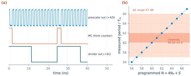
Two details matter. XSPICE’s digital elements default to 1 ns delays, which alone would eat the whole 1.0 ns budget of the critical loop, so every delay is set explicitly. And the analog-to-digital bridge passes through the unknown state on every edge; Verilog counts both 0 → x and x → 1 as rising edges, so the first version of the counter counted twice per cycle until the clk === 1'b1 test was added.
Figure 13.7 shows the result for twelve ratios, simulated as four dividers per run with the prescaler clocked at 2.44 GHz. For \(N_{div}\) = 61 (\(N_P\) = 15, \(S\) = 1), the prescaler divides by five once and by four fourteen times per frame, and the output period is exactly 61 input periods. All twelve ratios from 56 to 67 come out right: in every frame the prescaler divides by five \(S\) times and by four \(N_P - S\) times, and the output period equals \(N_{div}\) input periods to within 0.01, the rounding of the clock source’s period in the netlist. The prescaler draws 178 µW at 2.44 GHz.
A real design · The SG13G2 fractional-N PLL of Thiriloganathan et al.
An open-source 2.4 GHz fractional-N PLL in SG13G2 [106, 207] takes a different route. Its LC VCO runs directly at 2.4 GHz with a 10 MHz reference, and its whole divider, a fixed divide-by-4, a 4/5 prescaler with a modulo-7 counter (together 30 or 31) and a final divide-by-2 that squares the duty cycle, is written in Verilog, synthesized with Yosys and hardened with LibreLane, with a first-order delta-sigma modulator choosing between 240 and 248. The digital flow gives a DRC- and LVS-clean layout of the whole chain from a few hundred lines of code, which is a real advantage for an open-source design. The cost shows in three places: the fixed divide-by-4 in front of the dual-modulus stage makes the smallest step of the ratio 8 instead of 1, so the delta-sigma modulator’s quantization noise is larger; the first stage must toggle at 2.4 GHz in logic not designed for it; and there is no on-chip quadrature from the divider. The course chain keeps a custom CML stage at the VCO and a TSPC prescaler, and synthesizes only the counters, which run at 621 MHz or less.
13.5 Injection-locked and regenerative dividers
At millimetre waves the static dividers of Section 13.2 run out of speed or burn too much power: the nMOS CML divider stops at 14 GHz, and the HBT divider reaches 100 GHz only with 10.0 mW. Two families of analog dividers go further with less power.
Injection-locked dividers
An injection-locked frequency divider (ILFD) is an oscillator that runs near \(f_{in}/N\) and is pulled into exact step by the input. For division by two, the input is injected where a signal at twice the oscillation frequency acts on the oscillator, typically into the tail of a cross-coupled LC oscillator [141, 142]. The tail current, modulated at \(2f\), multiplies the switching of the pair at \(f\); the product contains a component at \(f\) whose phase follows the input, and that component locks the oscillator as an injected current would (Chapter 5 introduced the effect as injection pulling [71, 82]). The input can move only as far as the injected component can shift the oscillation frequency, which gives the lock range:
Key equation · Lock range of a tail-injected divide-by-two
\[\left(\frac{\Delta f_{in}}{f_{in}}\right)_{total} \approx \frac{2}{3}\,\frac{1}{Q}\,\frac{I_{inj}}{I_0}. \tag{13.8}\]\(I_0\) is the tail current, \(I_{inj}\) the amplitude of its modulation at \(f_{in}\), and \(Q\) the tank’s quality factor; the factor 2/3 holds for a pair that switches hard.
Derivation · Lock range of the tail-injected divider
Let the pair switch hard, so its differential output current is \(I_T(t)\,\mathrm{sgn}(v)\) with \(v = A\cos\theta\), \(\theta = \omega t + \varphi\), and \(I_T = I_0 + I_{inj}\cos 2\omega t\). The square wave \(\mathrm{sgn}(\cos\theta) = \tfrac{4}{\pi}(\cos\theta - \tfrac13\cos3\theta + \dots)\). The \(I_0\) term gives the oscillation current \(I_{osc} = (4/\pi)I_0\) at \(\omega\). The \(I_{inj}\) term mixes \(\cos2\omega t\) with \(\cos\theta\) and with \(\cos3\theta\); both products have a component at \(\omega\), \(\tfrac{2}{\pi}I_{inj}[\cos(\theta - 2\varphi) - \tfrac13\cos(\theta + 2\varphi)]\). Its part in quadrature with the oscillation is \(\tfrac{8}{3\pi}I_{inj}\sin2\varphi\), at most \(\tfrac{8}{3\pi}I_{inj}\). Adler’s result (Eq. 5.15) lets a quadrature current \(I_q\) shift the oscillation by \(\Delta\omega = (\omega_0/2Q)(I_q/I_{osc})\), so the output can be pulled by up to \((\omega_0/2Q)\cdot\tfrac{2}{3}I_{inj}/I_0\) either way. The input moves twice as far in hertz at twice the frequency, the same fraction; the total range is twice the one-sided one, Eq. (13.8).
Figure 13.8 checks Eq. (13.8) with a behavioural model: a 25 GHz tank (L = 200 pH, C = 203 fF) driven by a pair with a tanh characteristic and a 2 mA tail, integrated in the time domain for every combination of injection frequency and strength. With \(Q\) = 10 and \(I_{inj}/I_0\) = 0.3, the divider stays locked over 1.96 % of the input frequency, against 2.00 % from Eq. (13.8); with \(Q\) = 5, over 3.73 % against 4.00 %. Across all strengths the simulation stays within 9 % of the equation. The model is not a transistor-level design: it ignores the pair’s capacitance, the tank’s frequency dependence and the drop in injection efficiency of a real tail transistor at 50 GHz, all of which shrink the range [142].
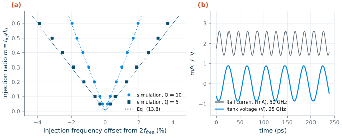
The narrow range is the ILFD’s weakness. A millimetre-wave VCO that tunes over ±5 % needs, by Eq. (13.8), \(I_{inj}/I_0 \ge 0.15\,Q\): with a tank Q of 10 that is more injection than the tail can supply. Practical ILFDs lower the tank Q, tune their tank together with the VCO’s, or add a calibration loop. In return they divide at frequencies where no static divider works, with a few milliwatts or less.
Regenerative (Miller) dividers
The regenerative divider, due to Miller [137], closes a loop around a mixer and a filter: the mixer multiplies the input at \(f_{in}\) by the output at \(f_{in}/2\), producing \(f_{in}/2\) and \(3f_{in}/2\); the filter keeps \(f_{in}/2\) and feeds it back. The loop sustains itself if its gain at \(f_{in}/2\) exceeds one. It has no resonance of its own and produces nothing without an input, so its range is set by the filter’s bandwidth and the mixer’s conversion gain, often much wider than an ILFD’s, at the cost of a mixer’s power. Both kinds suit the first divider of a millimetre-wave synthesizer, followed by static ECL or CML stages once the frequency has come down.
13.6 Divider noise and jitter
How divider noise enters the PLL
A divider in the feedback path adds phase noise \(\phi_{n,div}\) at its output. The loop compares the divided phase with the reference, so within its bandwidth it moves the VCO until the divider’s output follows the reference: the VCO acquires \(-N\phi_{n,div}\), where \(N\) is the ratio from the VCO to that divider’s output. Referred to the synthesizer output, the divider noise is multiplied by \(N\), like the reference noise (Chapter 12 derives the transfer functions). Outside the loop bandwidth the loop does nothing, and only the stages whose output is the output matter: in the course radio, the divide-by-two, whose output is the LO.
The first divide-by-two of the course chain plays both roles. Inside the loop bandwidth its noise is cancelled at the LO, because the LO is taken at the same point from which the feedback continues. Outside, its noise floor adds directly to the LO. The later stages, at the end of a chain of ratio \(N_{div}\) = 60–62, have their output noise multiplied by \(N_{div}\) at the LO within the loop bandwidth.
Additive jitter and the phase-noise floor
A divider’s noise is best described as a timing error of its output edges, its additive jitter. If every output edge is displaced by an independent random time of standard deviation \(\sigma_t\), the edges sample a white phase noise at the output frequency, and its single-sideband density is [144]
Key equation · Phase-noise floor of a divider with white edge jitter
\[\mathcal{L}_{floor} = 10\log_{10}\left(4\pi^2 f_{out}\,\sigma_t^2\right)\ \ \mathrm{dBc/Hz}. \tag{13.9}\]Referred to the PLL output, inside the loop bandwidth: \(\mathcal{L}_{out} = 4\pi^2 f_{out,PLL}^2\,\sigma_t^2/f_{out}\).
The edge jitter itself comes from the noise voltage at the output node at the moment it crosses its threshold, divided by how fast it crosses [145, 144]:
\[\sigma_t \approx \frac{\sigma_v}{SR}, \tag{13.10}\]with \(\sigma_v\) the rms noise voltage and \(SR\) the slew rate at the crossing. Fast edges and large node capacitances, which lower \(kT/C\) noise, make quiet dividers.
Estimating the jitter of the course divide-by-two
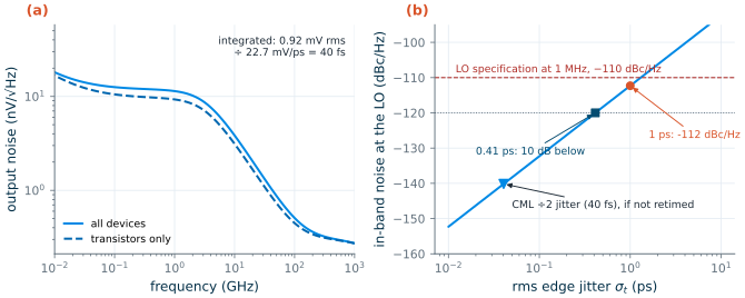
Neither ngspice nor Xyce has a periodic noise analysis (Chapter 2), so we estimate Eq. (13.10) from a small-signal analysis at the switching instant. The transient of Figure 13.3 gives the clock voltages at the moment the I output crosses zero: \(V_{CK}\) = 1.01 V and \(V_{\overline{CK}}\) = 0.494 V, 33.9 ps after the clock’s own crossing. A noise analysis of the master latch frozen at those clock voltages, with its inputs balanced by noiseless sources and the slave as its load, gives the output noise density of Figure 13.9a: 0.92 mV rms in total, 30 % of the power from the load resistors and the rest from the transistors. Divided by the slew rate of the transient at the crossing, 22.7 mV/ps, Eq. (13.10) gives σt ≈ 40 fs per output edge, and Eq. (13.9) a floor of −158 dBc/Hz at 2.4 GHz, −152 dBc/Hz when referred to the 4.8 GHz VCO.
The estimate has clear limits. It treats a moving waveform as a stationary bias point, integrates the noise over the whole band instead of the window in which the edge is decided, ignores the noise of the clock input and treats every edge as independent. It is good to a few decibels, not better. We tried to check it with ngspice’s transient noise sources across the load resistors, but 400 output periods of the PSP divider at 1 ps steps did not finish within half an hour; the frozen analysis is what remains. Even with a few decibels of error, the divider’s floor lies far below the VCO’s noise at the offsets that matter.
What the later stages may add
The stages after the divide-by-two matter inside the loop bandwidth. With the second form of Eq. (13.9), edge jitter \(\sigma_t\) on the 40 MHz output of the programmable divider appears at the 2.44 GHz LO as \(4\pi^2 f_{LO}^2\sigma_t^2/f_{ref}\): 1 ps rms gives −112 dBc/Hz (Figure 13.9b), as much as the course’s whole −110 dBc/Hz budget at 1 MHz; the divide-by-two’s 40 fs would give −140 dBc/Hz. To stay 10 dB below that budget, the divider’s output must jitter by less than 0.41 ps. Synthesized counters at a few hundred megahertz, with slow edges and supply noise from the digital circuits around them, are hard to hold to that. The usual cure is retiming: a flip-flop clocked by the 2.4 GHz divide-by-two output (or the prescaler output) re-samples the counter’s output, so its edges carry the jitter of a fast, clean stage instead [144, 11]. Chapter 12 adds the divider to the synthesizer’s noise budget.
13.7 The course divider chain
Table 13.2 collects the chain of Figure 13.1.
Table 13.2. The course divider chain in SG13G2 (typical models, 27 °C, 1.2 V). Numbers from the simulations of this chapter; the counters and the retiming flip-flop are not simulated at transistor level.
| Stage | Input | Circuit | Simulated performance | Power |
|---|---|---|---|---|
| Divide-by-two, I/Q generator | 4.80–4.97 GHz, sine from the VCO | tail-less CML, lv nMOS 6 µm, RL = 1 kΩ | divides from 100 mV at 4.8 GHz, up to 14 GHz; I/Q error 0.114°/mV of input offset; σt ≈ 40 fs, floor −158 dBc/Hz | 2.01 mW |
| CML-to-CMOS converter | 2.40–2.485 GHz | inverter or differential-to-single-ended stage | (not simulated) | |
| Dual-modulus prescaler | 2.40–2.485 GHz | ÷4/5, three TSPC flip-flops and an AOI21 | correct for Ndiv = 56–67 with the counters; a TSPC ÷2 alone toggles up to 7 GHz | 178 µW |
| Program and swallow counters | ≤ 621 MHz | Verilog, NP = 14–16, S = 0–3 (to be synthesized) | closed the loop with the prescaler in d_cosim | |
| Retiming flip-flop | 40 MHz data, 2.4 GHz clock | TSPC or CML flip-flop | (proposed, Section 13.6) |
For a millimetre-wave version of the synthesizer, the first stage would be the npn13G2 ECL divider (100 GHz, 10.0 mW) or an injection-locked divider, and the CML and TSPC stages would follow once the frequency has dropped below about 10 GHz.
Try it · The divider script
Every number in this chapter comes from
tools/figs/ch13_dividers.pyand its circuits in_ch13_cells.py:python3 tools/figs/ch13_dividers.pyredraws everything from the cached simulations,--resimreruns them (about 45 minutes, mostly the sensitivity sweeps). Three experiments: (1) inCML, lowervcmof the nominal design to 0.70 V and rerunsens --resim: where do \(f_{so}\) and the tip of the V move, and does the divider still self-oscillate? (2) ChangeP_MODto 8 andN_RANGEto 56–71 and rerunpsc --resim: does the Verilog counter still close the loop, and how much slower do the counters run? (3) Inpart_ilfd, add a quality factor of 20 toQS: does the lock range halve again, as Eq. (13.8) predicts?
- A divider divides phase as well as frequency, lowering phase noise by 20 log N; its first stage runs at the VCO frequency and sets the chain’s power, speed and, in the course radio, the I/Q accuracy.
- A CML divide-by-two is an injection-locked two-stage ring oscillator: its sensitivity curve is a V with its tip near twice the self-oscillation frequency. The course divider (tail-less, 6 µm, 1 kΩ) uses 2.01 mW, needs 100 mV at 4.8 GHz and toggles to 14 GHz; its I/Q error is about 0.11° per millivolt of input offset.
- SiGe ECL divides up to 100 GHz for 10.0 mW, 7.1 times faster than the nMOS CML; TSPC follows the first divide-by-two at 63.6 µW, but needs a rail-to-rail clock and has a minimum frequency.
- A 4/5 prescaler and a pulse-swallow counter give N = 4NP + S; only the prescaler runs fast, and the counters, written in Verilog and co-simulated with the transistor-level prescaler, cover the course’s 56–67.
- Injection-locked dividers reach millimetre waves on little power but lock over only about (2/3)(Iinj/I0)/Q; regenerative dividers trade power for range.
- Divider jitter inside the loop is multiplied by N: the course divide-by-two adds about 40 fs (a small-signal estimate), but the 40 MHz output of the chain must stay below 0.41 ps, which calls for retiming.
Further reading
- B. Razavi, Design of CMOS Phase-Locked Loops [11]: the chapter on dividers covers CML and TSPC dividers, dual-modulus prescalers and their timing, and divider noise, in more depth than this chapter; RF Microelectronics [6] gives the shorter radio-centred version.
- J. Lee and B. Razavi [143] on the CML divider as an injection-locked ring oscillator and its sensitivity curve; H.-M. Rein and M. Möller [140] on bipolar CML and ECL at the limits of speed.
- J. Yuan and C. Svensson [138], the TSPC paper, and J. Craninckx and M. Steyaert [139], a classic dual-modulus prescaler with a careful treatment of its critical loop.
- H. R. Rategh and T. H. Lee [141] and S. Verma, H. R. Rategh and T. H. Lee [142] on injection-locked dividers and their lock range; R. L. Miller [137] for the regenerative divider.
- S. Levantino et al. [144] on the phase noise of digital dividers, retiming included; S. Palermo’s ECEN 620 notes [2] for dividers in the context of the whole PLL.